Practical Deep Learnings For Coders - Part 1 Notes and Examples

deep learning

python

An update on my progress through part 1 of the fastai course.

Author

Vishal Bakshi

Published

June 1, 2023

Practical Deep Learning for Coders - Part 1

Vishal Bakshi

This notebook contains my notes (of course videos, example notebooks and book chapters) and exercises of Part 1 of the course Practical Deep Learning for Coders.

Lesson 1: Getting Started

Notebook Exercise

The first thing I did was to run through the lesson 1 notebook from start to finish. In this notebook, they download training and validation images of birds and forests then train an image classifier with 100% accuracy in identifying images of birds.

The first exercise is for us to create our own image classifier with our own image searches. I’ll create a classifier which accurately predicts an image of an alligator.

I’ll start by using their example code for getting images using DuckDuckGo image search:

# It's a good idea to ensure you're running the latest version of any libraries you need.
# `!pip install -Uqq <libraries>` upgrades to the latest version of <libraries>
# NB: You can safely ignore any warnings or errors pip spits out about running as root or incompatibilities
!pip install -Uqq fastai fastbook duckduckgo_search timm

from duckduckgo_search import ddg_images
from fastcore.all import *

def search_images(term, max_images=30):
    print(f"Searching for '{term}'")
    return L(ddg_images(term, max_results=max_images)).itemgot('image')

The search_images function takes a search term and max_images maximum number of images value. It prints out a line of text that it’s "Searching for" the term and returns an L object with the image URL.

The ddg_images function returns a list of JSON objects containing the title, image URL, thumbnail URL, height, width and source of the image.

search_object = ddg_images('alligator', max_results=1)
search_object

/usr/local/lib/python3.9/dist-packages/duckduckgo_search/compat.py:60: UserWarning: ddg_images is deprecated. Use DDGS().images() generator
  warnings.warn("ddg_images is deprecated. Use DDGS().images() generator")
/usr/local/lib/python3.9/dist-packages/duckduckgo_search/compat.py:64: UserWarning: parameter page is deprecated
  warnings.warn("parameter page is deprecated")
/usr/local/lib/python3.9/dist-packages/duckduckgo_search/compat.py:66: UserWarning: parameter max_results is deprecated
  warnings.warn("parameter max_results is deprecated")

[{'title': 'The Creature Feature: 10 Fun Facts About the American Alligator | WIRED',
  'image': 'https://www.wired.com/wp-content/uploads/2015/03/Gator-2.jpg',
  'thumbnail': 'https://tse4.mm.bing.net/th?id=OIP.FS96VErnOXAGSWU092I_DQHaE8&pid=Api',
  'url': 'https://www.wired.com/2015/03/creature-feature-10-fun-facts-american-alligator/',
  'height': 3456,
  'width': 5184,
  'source': 'Bing'}]

Wrapping this list in L object and calling .itemgot('image') on it extracts URL value associated with the image key in the JSON object.

L(search_object).itemgot('image')

(#1) ['https://www.wired.com/wp-content/uploads/2015/03/Gator-2.jpg']

Next, they provide some code to download the image to a destination filename and view the image:

urls = search_images('alligator', max_images=1)

from fastdownload import download_url
dest = 'alligator.jpg'
download_url(urls[0], dest, show_progress=False)

from fastai.vision.all import *
im = Image.open(dest)
im.to_thumb(256,256)

Searching for 'alligator'

For my not-alligator images, I’ll use images of a swamp.

download_url(search_images('swamp photos', max_images=1)[0], 'swamp.jpg', show_progress=False)
Image.open('swamp.jpg').to_thumb(256,256)

Searching for 'swamp photos'

/usr/local/lib/python3.9/dist-packages/duckduckgo_search/compat.py:60: UserWarning: ddg_images is deprecated. Use DDGS().images() generator
  warnings.warn("ddg_images is deprecated. Use DDGS().images() generator")
/usr/local/lib/python3.9/dist-packages/duckduckgo_search/compat.py:64: UserWarning: parameter page is deprecated
  warnings.warn("parameter page is deprecated")
/usr/local/lib/python3.9/dist-packages/duckduckgo_search/compat.py:66: UserWarning: parameter max_results is deprecated
  warnings.warn("parameter max_results is deprecated")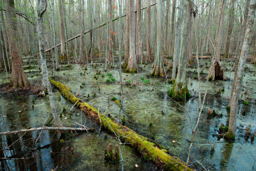

In the following code, I’ll search for both terms, alligator and swamp and store the images in alligator_or_not/alligator and alligator_or_not/swamp paths, respectively.

The parents=TRUE argument creates any intermediate parent directories that don’t exist (in this case, the alligator_or_not directory). The exist_ok=TRUE argument suppresses the FileExistsError and does nothing.

searches = 'swamp','alligator'
path = Path('alligator_or_not')
from time import sleep

for o in searches:
    dest = (path/o)
    dest.mkdir(exist_ok=True, parents=True)
    download_images(dest, urls=search_images(f'{o} photo'))
    sleep(10)  # Pause between searches to avoid over-loading server
    download_images(dest, urls=search_images(f'{o} sun photo'))
    sleep(10)
    download_images(dest, urls=search_images(f'{o} shade photo'))
    sleep(10)
    resize_images(path/o, max_size=400, dest=path/o)

Searching for 'swamp photo'
Searching for 'swamp sun photo'
Searching for 'swamp shade photo'
Searching for 'alligator photo'
Searching for 'alligator sun photo'
Searching for 'alligator shade photo'

Next, I’ll train my model using the code they have provided.

The get_image_files function is a fastai function which takes a Path object and returns an L object with paths to the image files.

type(get_image_files(path))

fastcore.foundation.L

get_image_files(path)

(#349) [Path('alligator_or_not/swamp/1b3c3a61-0f7f-4dc2-a704-38202d593207.jpg'),Path('alligator_or_not/swamp/9c9141f2-024c-4e26-b343-c1ca1672fde8.jpeg'),Path('alligator_or_not/swamp/1340dd85-5d98-428e-a861-d522c786c3d7.jpg'),Path('alligator_or_not/swamp/2d3f91dc-cc5f-499b-bec6-7fa0e938fb13.jpg'),Path('alligator_or_not/swamp/84afd585-ce46-4016-9a09-bd861a5615db.jpg'),Path('alligator_or_not/swamp/6222f0b6-1f5f-43ec-b561-8e5763a91c61.jpg'),Path('alligator_or_not/swamp/a71c8dcb-7bbb-4dba-8ae6-8a780d5c27c6.jpg'),Path('alligator_or_not/swamp/bbd1a832-a901-4e8f-8724-feac35fa8dcb.jpg'),Path('alligator_or_not/swamp/45b358b3-1a12-41d4-8972-8fa98b2baa52.jpg'),Path('alligator_or_not/swamp/cf664509-8eb6-42c8-9177-c17f48bc026b.jpg')...]

The fastai parent_label function takes a Path object and returns a string of the file’s parent folder name.

parent_label(Path('alligator_or_not/swamp/18b55d4f-3d3b-4013-822b-724489a23f01.jpg'))

'swamp'

Some image files that are downloaded may be corrupted, so they have provided a verify_images function to find images that can’t be opened. Those images are then removed (unlinked) from the path.

failed = verify_images(get_image_files(path))
failed.map(Path.unlink)
len(failed)

failed

(#1) [Path('alligator_or_not/alligator/1eb55508-274b-4e23-a6ae-dbbf1943a9d1.jpg')]

dls = DataBlock(
    blocks=(ImageBlock, CategoryBlock),
    get_items=get_image_files,
    splitter=RandomSplitter(valid_pct=0.2, seed=42),
    get_y=parent_label,
    item_tfms=[Resize(192, method='squish')]
).dataloaders(path, bs=32)

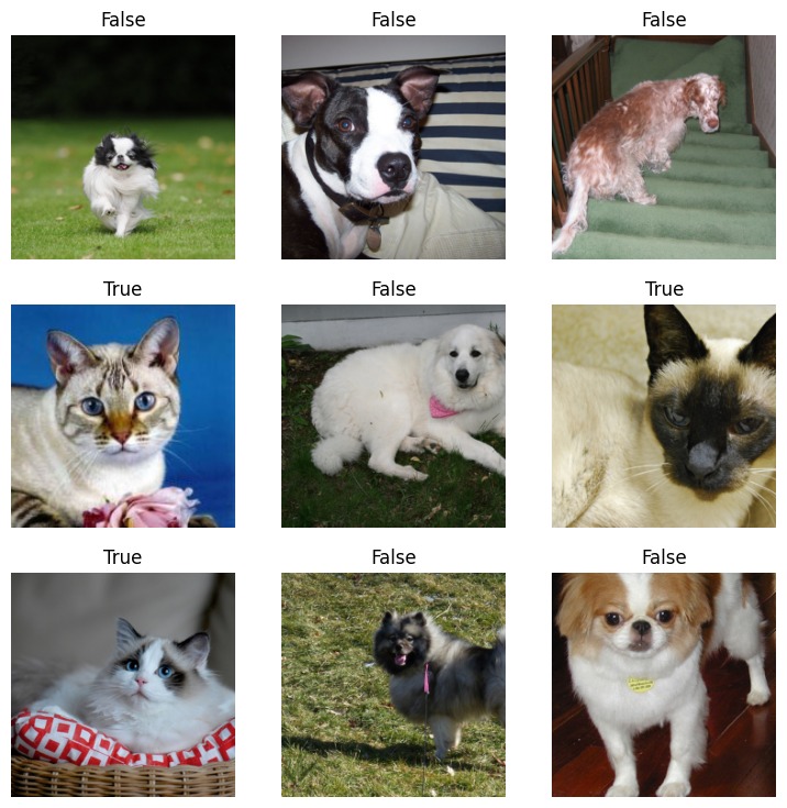
dls.show_batch(max_n=6)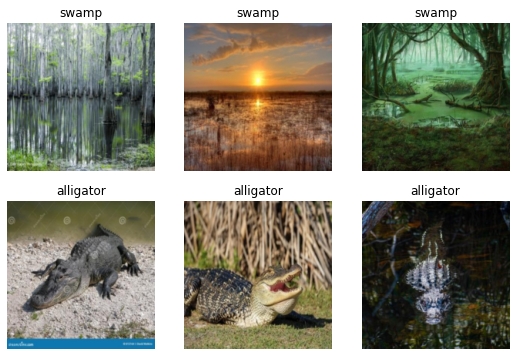

I’ll train the model using their code which uses the resnet18 image classification model, and fine_tunes it for 3 epochs.

learn = vision_learner(dls, resnet18, metrics=error_rate)
learn.fine_tune(3)

/usr/local/lib/python3.9/dist-packages/torchvision/models/_utils.py:208: UserWarning: The parameter 'pretrained' is deprecated since 0.13 and will be removed in 0.15, please use 'weights' instead.
  warnings.warn(
/usr/local/lib/python3.9/dist-packages/torchvision/models/_utils.py:223: UserWarning: Arguments other than a weight enum or `None` for 'weights' are deprecated since 0.13 and will be removed in 0.15. The current behavior is equivalent to passing `weights=ResNet18_Weights.IMAGENET1K_V1`. You can also use `weights=ResNet18_Weights.DEFAULT` to get the most up-to-date weights.
  warnings.warn(msg)
Downloading: "https://download.pytorch.org/models/resnet18-f37072fd.pth" to /root/.cache/torch/hub/checkpoints/resnet18-f37072fd.pth

epoch	train_loss	valid_loss	error_rate	time
0	0.690250	0.171598	0.043478	00:03

epoch	train_loss	valid_loss	time
0	0.127188	0.001747	00:02
1	0.067970	0.006409	00:02
2	0.056453	0.004981	00:02

The accuracy is 100%.

Next, I’ll test the model as they’ve done in the lesson.

PILImage.create('alligator.jpg').to_thumb(256,256)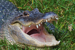

is_alligator,_,probs = learn.predict(PILImage.create('alligator.jpg'))
print(f"This is an: {is_alligator}.")
print(f"Probability it's an alligator: {probs[0]:.4f}")

This is an: alligator.
Probability it's an alligator: 1.0000

Video Notes

In this section, I’ll take notes while I watch the lesson 1 video.

This is the fifth version of the course!
What seemed impossible in 2015 (image recognition of a bird) is now free and something we can build in 2 minutes.
All models need numbers as their inputs. Images are already stored as numbers in computers. [PixSpy] allows you to (among other things) view the color of each pixel in an image file.
A DataBlock gives fastai all the information it needs to create a computer vision model.
Creating really interesting, real, working programs with deep learning is something that doesn’t take a lot of code, math, or more than a laptop computer. It’s pretty accessible.
Deep Learning models are doing things that very few, if any of us, believed would be possible to do by computers in our lifetime.
See the Practical Data Ethics course as well.
Meta Learning: How To Learn Deep Learning And Thrive In The Digital World.
Books on learning/education:
- Mathematician’s Lament by Paul Lockhart
- Making Learning Whole by David Perkins
Why are we able to create a bird-recognizer in a minute or two? And why couldn’t we do it before?
- 2012: Project looking at 5-year survival of breast cancer patients, pre-deep learning approach
  - Assembled a team to build ideas for thousands of features that required a lot of expertise, took years.
  - They fed these features into a logistic regression model to predict survival.
  - Neural networks don’t require us to build these features, they build them for us.
- 2015: Matthew D. Zeiler and Rob Fergus looked inside a neural network to see what it had learned.
  - We don’t give it features, we ask it to learn features.
  - The neural net is the basic function used in deep learning.
  - You start with a random neural network, feed it examples and you have it learn to recognize things.
  - The deeper you get, the more sophisticated the features it can find are.
  - What we’re going to learn is how neural networks do this automatically.
  - This is the key difference in why we can now do things that we couldn’t previously conceive of as possible.
An image recognizer can also be used to classify sounds (pictures of waveforms).
Turning time series into pictures for image classification.
fastai is built on top of PyTorch.
!pip install -Uqq fastai to update.
Always view your data at every step of building a model.
For computer vision algorithms you don’t need particularly big images.
For big images, most of the time is taken up opening it, the neural net on the GPU is must faster.
The main thing you’re going to try and figure out is how do I get this data into my model?
DataBlock
- blocks=(ImageBlock, CategoryBlock): ImageBlock is the type of input to the model, CategoryBlock is the type of model output
- get_image_files(path) returns a list of all image files in a path.
- It’s critical that you put aside some data for testing the accuracy of your model (validation set) with something like RandomSplitter for the splitter parameter.
- get_y tells fastai how to get the correct label for the photo.
- Most computer vision architectures need all of your inputs to be the same size, using Resize (either crop out a piece in the middle or squish the image) for the parameter item_tfms.
- DataLoaders contains iterators that PyTorch can run through to grab batches of your data to feed the training algorithm.
- show_batch shows you a batch of input/label pairs.
- A Learner combines a model (the actual neural network that we are training) and the data we use to train it with.
- PyTorch Image Models (timm).
- resnet has already been trained to recognize over 1 million images of over 1000 different types. fastai downloads this so you can start with a neural network that can do a lot.
- fine_tune takes those pretrained weights downloaded for you and adjusts them in a carefully controlled way to teach the model differences between your dataset and what it was originally trained for.
- You pass .predict an image, which is how you would deploy your model, returns whether it’s a bird or not as a string, integer and probability of whether it’s a bird (in this example).

In the code blocks below, I’ll train the different types of models presented in the video lesson.

Image Segmentation

from fastai.vision.all import *

path = untar_data(URLs.CAMVID_TINY)
dls = SegmentationDataLoaders.from_label_func(
    path, bs = 8, fnames = get_image_files(path/"images"),
    label_func = lambda o: path/'labels'/f'{o.stem}_P{o.suffix}',
    codes = np.loadtxt(path/'codes.txt', dtype=str)
)

learn = unet_learner(dls, resnet34)
learn.fine_tune(8)

/usr/local/lib/python3.9/dist-packages/torchvision/models/_utils.py:208: UserWarning: The parameter 'pretrained' is deprecated since 0.13 and will be removed in 0.15, please use 'weights' instead.
  warnings.warn(
/usr/local/lib/python3.9/dist-packages/torchvision/models/_utils.py:223: UserWarning: Arguments other than a weight enum or `None` for 'weights' are deprecated since 0.13 and will be removed in 0.15. The current behavior is equivalent to passing `weights=ResNet34_Weights.IMAGENET1K_V1`. You can also use `weights=ResNet34_Weights.DEFAULT` to get the most up-to-date weights.
  warnings.warn(msg)
Downloading: "https://download.pytorch.org/models/resnet34-b627a593.pth" to /root/.cache/torch/hub/checkpoints/resnet34-b627a593.pth

epoch	train_loss	valid_loss	time
0	3.454409	3.015761	00:06

epoch	train_loss	valid_loss	time
0	1.928762	1.719756	00:02
1	1.649520	1.394089	00:02
2	1.533350	1.344445	00:02
3	1.414438	1.279674	00:02
4	1.291168	1.063977	00:02
5	1.174492	0.980055	00:02
6	1.073124	0.931532	00:02
7	0.992161	0.922516	00:02

learn.show_results(max_n=3, figsize=(7,8))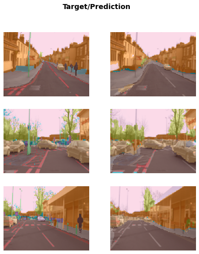

It’s amazing how many it’s getting correct because this model was trained in about 24 seconds using a tiny amount of data.

I’ll take a look at the codes out of curiousity, which is an array of string elements describing different objects in view.

np.loadtxt(path/'codes.txt', dtype=str)

array(['Animal', 'Archway', 'Bicyclist', 'Bridge', 'Building', 'Car',
       'CartLuggagePram', 'Child', 'Column_Pole', 'Fence', 'LaneMkgsDriv',
       'LaneMkgsNonDriv', 'Misc_Text', 'MotorcycleScooter', 'OtherMoving',
       'ParkingBlock', 'Pedestrian', 'Road', 'RoadShoulder', 'Sidewalk',
       'SignSymbol', 'Sky', 'SUVPickupTruck', 'TrafficCone',
       'TrafficLight', 'Train', 'Tree', 'Truck_Bus', 'Tunnel',
       'VegetationMisc', 'Void', 'Wall'], dtype='<U17')

Tabular Analysis

from fastai.tabular.all import *
path = untar_data(URLs.ADULT_SAMPLE)

dls = TabularDataLoaders.from_csv(path/'adult.csv', path=path, y_names='salary',
                                  cat_names = ['workclass', 'education', 'marital-status', 'occupation',
                                               'relationship', 'race'],
                                  cont_names = ['age', 'fnlwgt', 'education-num'],
                                  procs = [Categorify, FillMissing, Normalize])

dls.show_batch()

	workclass	education	marital-status	occupation	relationship	race	education-num_na	age	fnlwgt	education-num	salary
0	State-gov	Some-college	Divorced	Adm-clerical	Own-child	White	False	42.0	138162.000499	10.0	<50k
1	Private	HS-grad	Married-civ-spouse	Other-service	Husband	Asian-Pac-Islander	False	40.0	73025.003080	9.0	<50k
2	Private	Assoc-voc	Married-civ-spouse	Prof-specialty	Wife	White	False	36.0	163396.000571	11.0	>=50k
3	Private	HS-grad	Never-married	Sales	Own-child	White	False	18.0	110141.999831	9.0	<50k
4	Self-emp-not-inc	12th	Divorced	Other-service	Unmarried	White	False	28.0	33035.002716	8.0	<50k
5	?	7th-8th	Separated	?	Own-child	White	False	50.0	346013.994175	4.0	<50k
6	Self-emp-inc	HS-grad	Never-married	Farming-fishing	Not-in-family	White	False	36.0	37018.999571	9.0	<50k
7	State-gov	Masters	Married-civ-spouse	Prof-specialty	Husband	White	False	37.0	239409.001471	14.0	>=50k
8	Self-emp-not-inc	Doctorate	Married-civ-spouse	Prof-specialty	Husband	White	False	50.0	167728.000009	16.0	>=50k
9	Private	HS-grad	Married-civ-spouse	Tech-support	Husband	White	False	38.0	247111.001513	9.0	>=50k

For tabular models, there’s not generally going to be a pretrained model that already does something like what you want because every table of data is very different, so generally it doesn’t make too much sense to fine_tune a tabular model.

learn = tabular_learner(dls, metrics=accuracy)
learn.fit_one_cycle(2)

epoch	train_loss	valid_loss	accuracy	time
0	0.373780	0.365976	0.832770	00:06
1	0.356514	0.358780	0.833999	00:05

Collaborative Filtering

The basis of most recommendation systems.

from fastai.collab import *
path = untar_data(URLs.ML_SAMPLE)
dls = CollabDataLoaders.from_csv(path/'ratings.csv')

dls.show_batch()

	userId	movieId	rating
0	457	457	3.0
1	407	2959	5.0
2	294	356	4.0
3	78	356	5.0
4	596	3578	4.5
5	547	541	3.5
6	105	1193	4.0
7	176	4993	4.5
8	430	1214	4.0
9	607	858	4.5

There’s actually no pretrained collaborative filtering model so we could use fit_one_cycle but fine_tune works here as well.

learn = collab_learner(dls, y_range=(0.5, 5.5))
learn.fine_tune(10)

epoch	train_loss	valid_loss	time
0	1.498450	1.417215	00:00

epoch	train_loss	valid_loss	time
0	1.375927	1.357755	00:00
1	1.274781	1.176326	00:00
2	1.033917	0.870168	00:00
3	0.810119	0.719341	00:00
4	0.704180	0.679201	00:00
5	0.640635	0.667121	00:00
6	0.623741	0.661391	00:00
7	0.620811	0.657624	00:00
8	0.606947	0.656678	00:00
9	0.605081	0.656613	00:00

learn.show_results()

	userId	movieId	rating	rating_pred
0	15.0	35.0	4.5	3.886339
1	68.0	64.0	5.0	3.822170
2	62.0	33.0	4.0	3.088149
3	39.0	91.0	4.0	3.788227
4	37.0	7.0	5.0	4.434169
5	38.0	98.0	3.5	4.380877
6	3.0	25.0	3.0	3.443295
7	23.0	13.0	2.0	3.220192
8	15.0	7.0	4.0	4.306846

Note: RISE turnes your notebook into a presentation.

Generally speaking, if it’s something that a human can do reasonably quickly, even an expert human (like look at a Go board and decide if it’s a good board or not) then that’s probably something that deep learning will probably be good at. If it’s something that takes logical thought process over time, particularly if it’s not based on much data, deep learning probably won’t do that well.

The first neural network was built in 1957. The basic ideas have not changed much at all.

What’s going on in these models?

Arthur Samuel in late 1950s invented Machine Learning.
Normal program: input -> program -> results.
Machine Learning model: input and weights (parameters) -> model -> results.
- The model is a mathematical function that takes the input, multiplies them with one set of weights and adds them up, then does that again for a second set of weights, and so forth.
- It takes all of the negative numbers and replaces them with 0.
- It takes all those numbers as inputs to the next layer.
- And it repeats a few times.
Weights start out as being random.
A more useful workflow: input/weights -> model -> results -> loss -> update weights.
The loss is a number that says how good the results were.
We need a way to come up with a new set of weights that are a bit better than the current weights.
“bit better” weights means it makes the loss a bit better.
If we make it a little bit better a few times, it’ll eventually get good.
Neural nets proven to solve any computable function (i.e. it’s flexible enough to update weights until the results are good).
“Generate artwork based on someone’s twitter bio” is a computable function.
Once we’ve finished the training procedure we don’t the loss and the weights can be integrated into the model.
We end up with inputs -> model -> results which looks like our original idea of a program.
Deploying a model will have lots of tricky details but there will be one line of code which says learn.predict which takes an input and provides results.
The most important thing to do is experiment.

Book Notes

Chapter 1: Your Deep Learning Journey In this section, I’ll take notes while I read Chapter 1 in the textbook.

Deep Learning is for Everyone

What you don’t need for deep learning: lots of math, lots of data, lots of expensive computers.
Deep learning is a computer technique to extract and transform data by using multiple layers of neural networks. Each of these layers takes its inputs from previous layers and progressively refines them. The layers are trained by algorithms that minimize their errors and improve their accuracy. In this way, the network learns to perform a specified task.

Neural Networks: A Brief History

Warren McCulloch and Walter Pitts developed a mathematical model of an artificial neuron in 1943.
Most of Pitt’s famous work was done while he was homeless.
Psychologist Frank Rosenblatt further developed the artificial neuron to give it the ability to learn and built the first device that used these principles, the Mark I Perceptron, which was able to recognize simple shapes.
Marvin Minsky and Seymour Papert wrote a book about the Perceptron and showed that using multiple layers of the devices would allow the limitations of a single layer to be addressed.
The 1986 book Parallel Distributed Processing (PDP) by David Rumelhart, James McClelland, and the PDP Research Group defined PDP as requiring the following:
- A set of processing units.
- A state of activation.
- An output function for each unit.
- A pattern of connectivity among units.
- A propogation rule for propagating patterns of activities through the network of connectivities.
- An activation rule for combining the inputs impinging on a unit with the current state of that unit to produce an output for the unit.
- A learning rule whereby patterns of connectivity are modified by experience.
- An environment within which the system must operate.

How to Learn Deep Learning

The hardest part of deep learning is artisanal: how do you know if you’ve got enough data, whether it is in the right format, if your model is training properly, and, if it’s not, what you should do about it?

from fastai.vision.all import *
path = untar_data(URLs.PETS)/'images'

def is_cat(x): return x[0].isupper()
dls = ImageDataLoaders.from_name_func(
    path,
    get_image_files(path),
    valid_pct=0.2,
    seed=42,
    label_func=is_cat,
    item_tfms=Resize(224)
)

dls.show_batch()

100.00% [811712512/811706944 00:11<00:00]

learn = cnn_learner(dls, resnet34, metrics=error_rate)
learn.fine_tune(1)

/usr/local/lib/python3.10/dist-packages/fastai/vision/learner.py:288: UserWarning: `cnn_learner` has been renamed to `vision_learner` -- please update your code
  warn("`cnn_learner` has been renamed to `vision_learner` -- please update your code")
/usr/local/lib/python3.10/dist-packages/torchvision/models/_utils.py:208: UserWarning: The parameter 'pretrained' is deprecated since 0.13 and may be removed in the future, please use 'weights' instead.
  warnings.warn(
/usr/local/lib/python3.10/dist-packages/torchvision/models/_utils.py:223: UserWarning: Arguments other than a weight enum or `None` for 'weights' are deprecated since 0.13 and may be removed in the future. The current behavior is equivalent to passing `weights=ResNet34_Weights.IMAGENET1K_V1`. You can also use `weights=ResNet34_Weights.DEFAULT` to get the most up-to-date weights.
  warnings.warn(msg)
Downloading: "https://download.pytorch.org/models/resnet34-b627a593.pth" to /root/.cache/torch/hub/checkpoints/resnet34-b627a593.pth
100%|██████████| 83.3M/83.3M [00:00<00:00, 162MB/s]

epoch	train_loss	valid_loss	error_rate	time
0	0.140327	0.019135	0.007442	01:05

0.00% [0/1 00:00<?]

epoch	train_loss	valid_loss	error_rate	time

4.17% [1/24 00:01<00:34]

epoch	train_loss	valid_loss	error_rate	time
0	0.070464	0.024966	0.006766	01:00

The error rate is the proportion of images that were incorrectly identified.

Check this model actually works with an image of a dog or cat. I’ll download a picture from google and use it for prediction:

import ipywidgets as widgets
uploader = widgets.FileUpload()
uploader

im = PILImage.create(uploader.data[0])
is_cat, _, probs = learn.predict(im)
im.to_thumb(256)

print(f'Is this a cat?: {is_cat}.')
print(f"Probability it's a cat: {probs[1].item():.6f}")

Is this a cat?: True.
Probability it's a cat: 1.000000

What is Machine Learning?

A traditional program: inputs -> program -> results.
In 1949, IBM researcher Arthur Samuel started working on machine learning. His basic idea was this: instead of telling the computer the exact steps required to solve a problem, show it examples of the problem to solve, and let it figure out how to solve it itself.
In 1961 his checkers-playing program had learned so much that it beat the Connecticut state champion.
Weights are just variables and a weight assignment is a particular choice of values for those variables.
The program’s inputs are values that it processes in order to produce its results (for instance, taking image pixels as inputs, and returning the classification “dog” as a result).
Because the weights affect the program, they are in a sense another kind of input.
A program using weight assignment: inputs and weights -> model -> results.
A model is a special kind of program, on that can do many different things depending on the weights.
Weights = parameters, with the term “weights” reserved for a particulat type of model parameter.
Learning would become entirely automatic when the adjustment of the weights was also automatic.
Training a maching learning model: inputs and weights -> model -> results -> performance -> update weights.
results are different than the performance of a model.
Using a trained model as a program -> inputs -> model -> results.
maching learning is the training of programs developed by allowing a computer to learn from its experience, rather than through manually coding the individual steps.

What is a Neural Network?

Neural networks is a mathematical function that can solve any problem to any level of accuracy.
Stochastic Gradient Descent (SGD) is a completely general way to update the weights of a neural network, to make it improve at any given task.
Image classification problem:
- Our inputs are the images.
- Our weights are the weights in the neural net.
- Our model is a neural net.
- Our results are the values that are calculated by the neural net, like “dog” or “cat”.

A Bit of Deep Learning Jargon

The functional form of the model is called its architecture.
The weights are called parameters.
The predictions are calculated from the independent variable, which is the data not including the labels.
The results or the model are called predictions.
The measure of performance is called the loss.
The loss depends not only on the predictions, but also on the correct labels (also known as targets or the dependent variable).
Detailed training loop: inputs and parameters -> architecture -> predictions (+ labels) -> loss -> update parameters.

Limitations Inherent to Machine Learning

A model cannot be created without data.
A model can learn to operate on only the patterns seen in the input data used to train it.
This learning approach creates only predictions, not recommended actions.
It’s not enough to just have examples of input data, we need labels for that data too.
Positive feedback loop: the more the model is used, the more biased the data becomes, making the model even more biased, and so forth.

How Our Image Recognizer Works

item_tfms are applied to each item while batch_tfms are applied to a batch of items at a time using the GPU.
A classification model attempts to predict a class, or category.
A regression model is one that attempts to predict one or more numeric quantities, such as temperature or location.
The parameter seed=42 sets the random seed to the same value every time we run this code, which means we get the same validation set every time we run it. This way, if we change our model and retrain it, we know that any differences are due to the changes to the model, not due to having a different random validation set.
We care about how well our model works on previously unseen images.
The longer you train for, the better your accuracy will get on the training set; the validation set accuracy will also improve for a while, but eventually it will start getting worse as the model starts to memorize the training set rather than finding generalizable underlying patterns in the data. When this happens, we say that the model is overfitting.
Overfitting is the single most important and challenging issue when training for all machine learning practitioners, and all algorithms.
You should only use methods to avoid overfitting after you have confirmed that overfitting is occurring (i.e., if you have observed the validation accuracy getting worse during training)
fastai defaults to valid_pct=0.2.
Models using architectures with more layers take longer to train and are more prone to overfitting, on the other hand, when using more data, they can be quite a bit more accurate.
A metric is a function that measures the quality of the model’s predictions using the validation set.
error_rate tells you what percentage of inputs in the validation set are being classified incorrectly.
accuracy = 1.0 - error_rate.
The entire purpose of loss is to define a “measure of performance” that the training system can use to update weights automatically. A good choice for loss is a choice that is easy for stochastic gradient descent to use. But a metric is defined for human consumption, so a good metric is one that is easy for you to understand.
A model that has weights that have already been trained on another dataset is called a pretrained model.
When using a pretrained model, cnn_learner will remove the last layer and replace it with one or more new layers with randomized weights. This last part of the model is known as the head.
Using a pretrained model for a task different from what is was originally trained for is known as transfer learning.
The architecture only describes a template for a mathematical function; it doesn’t actually do anything until we provide values for the millions of parameters it contains.
To fit a model, we have to provide at least one piece of information: how many times to look at each image (known as number of epochs).
fit will fit a model (i.e., look at images in the training set multiple times, each time updating the parameters to make the predictions closer and closer to the target labels).
Fine-Tuning: a transfer learning technique that updates the parameters of a pretrained model by training for additional epochs using a different task from that used for pretraining.
fine_tune has a few parameters you can set, but in the default form it does two steps:
- Use one epoch to fit just those parts of the model necessary to get the new random head to work correctly with your dataset.
- Use the number of epochs requested when calling the method to fit the entire model, updating the weights of the later layers (especially the head) faster than the earlier layers (which don’t require many changes from the pretrained weights).
The head of the model is the part that is newly added to be specific to the new dataset.
An epoch is one complete pass through the dataset.

What Our Image Recognizer Learned

When we fine tune our pretrained models, we adapt what the last layers focus on to specialize on the problem at hand.

Image Recognizers Can Tackle Non-Image Tasks

A lot of things can be represented as images.
Sound can be converted to a spectogram.
Times series data can be created into an image using Gramian Angular Difference Field (GADF).
If the human eye can recognize categories from the images, then a deep learning model should be able to do so too.

Jargon Recap

Term	Meaning
Label	The data that we’re trying to predict
Architecture	The template of the model that we’re trying to fit; i.e., the actual mathematical function that we’re passing the input data and parameters to
Model	The combination of the architecture with a particular set of parameters
Parameters	The values in the model that change what task it can do and that are updated through model training
Fit	Update the parameters of the model such that the predictions of the model using the input data match the target labels
Train	A synonym for fit
Pretrained Model	A model that has already been trained, generally using a large dataset, and will be fine-tuned
Fine-tune	Update a pretrained model for a different task
Epoch	One complete pass through the input data
Loss	A measure of how good the model is, chosen to drive training via SGD
Metric	A measurement of how good the model is using the validation set, chosen for human consumption
Validation set	A set of data held out from training, used only for measuring how good the model is
Training set	The data used for fitting the model; does not include any data from the validation set
Overfitting	Training a model in such a way that it remembers specific features of the input data, rather than generalizing wel to data not seen during training
CNN	Convolutional neural network; a type of neural network that works particularly well for computer vision tasks

Deep Learning is Not Just for Image Classification

Segmentation
Natural language processing (see below)
Tabular (see Adults income classification above)
Collaborative filtering (see MovieLens ratings predictor above)
Start by using one of the cut-down dataset versions and later scale up to the full-size version. This is how the world’s top practitioners do their modeling in practice; they do most of their experimentation and prototyping with subsets of their data, and use the full dataset only when they have a good understanding of what they have to do.

Validation Sets and Test Sets

If the model makes an accurate prediction for a data item, that should be because it has learned characteristics of that kind of item, and not because the model has been shaped by actually having seen that particular item.
Hyperparameters: various modeling choices regarding network architecture, learning rates, data augmentation strategies, and other factors.
We, as modelers, are evaluating the model by looking at predictions on the validation data when we decide to explore new hyperparameter values and we are in danger of overfitting the validation data through human trial and error and exploration.
The test set can be used only to evaluate the model at the very end of our efforts.
Training data is fully exposed to training and modeling processes, validation data is less exposed and test data is fully hidden.
The test and validation sets should have enough data to ensure that you get a good estimate of your accuracy.
The discipline of the test set helps us keep ourselves intellectually honest.
It’s a good idea for you to try out a simple baseline model yourself, so you know what a really simply model can achieve.

Use Judgment in Defining Test Sets

A key property of the validation and test sets is that they must be representative of the new data you will see in the future.
As an example, for time series data, use earlier dates for training set and later more recent dates as validation set
The data you will be making predictions for in production may be qualitatively different from the data you have to train your model with.

from fastai.text.all import *

# I'm using IMDB_SAMPLE instead of the full IMDB dataset since it either takes too long or
# I get a CUDA Out of Memory error if the batch size is more than 16 for the full dataset
# Using a batch size of 16 with the sample dataset works fast
dls = TextDataLoaders.from_csv(
    path=untar_data(URLs.IMDB_SAMPLE),
    csv_fname='texts.csv',
    text_col=1,
    label_col=0,
    bs=16)

dls.show_batch()

	text	category
0	xxbos xxmaj raising xxmaj victor xxmaj vargas : a xxmaj review \n\n xxmaj you know , xxmaj raising xxmaj victor xxmaj vargas is like sticking your hands into a big , xxunk bowl of xxunk . xxmaj it 's warm and gooey , but you 're not sure if it feels right . xxmaj try as i might , no matter how warm and gooey xxmaj raising xxmaj victor xxmaj vargas became i was always aware that something did n't quite feel right . xxmaj victor xxmaj vargas suffers from a certain xxunk on the director 's part . xxmaj apparently , the director thought that the ethnic backdrop of a xxmaj latino family on the lower east side , and an xxunk storyline would make the film critic proof . xxmaj he was right , but it did n't fool me . xxmaj raising xxmaj victor xxmaj vargas is	negative
1	xxbos xxup the xxup shop xxup around xxup the xxup corner is one of the xxunk and most feel - good romantic comedies ever made . xxmaj there 's just no getting around that , and it 's hard to actually put one 's feeling for this film into words . xxmaj it 's not one of those films that tries too hard , nor does it come up with the xxunk possible scenarios to get the two protagonists together in the end . xxmaj in fact , all its charm is xxunk , contained within the characters and the setting and the plot … which is highly believable to xxunk . xxmaj it 's easy to think that such a love story , as beautiful as any other ever told , * could * happen to you … a feeling you do n't often get from other romantic comedies	positive
2	xxbos xxmaj now that xxmaj che(2008 ) has finished its relatively short xxmaj australian cinema run ( extremely limited xxunk screen in xxmaj xxunk , after xxunk ) , i can xxunk join both xxunk of " at xxmaj the xxmaj movies " in taking xxmaj steven xxmaj soderbergh to task . \n\n xxmaj it 's usually satisfying to watch a film director change his style / subject , but xxmaj soderbergh 's most recent stinker , xxmaj the xxmaj girlfriend xxmaj xxunk ) , was also missing a story , so narrative ( and editing ? ) seem to suddenly be xxmaj soderbergh 's main challenge . xxmaj strange , after 20 - odd years in the business . xxmaj he was probably never much good at narrative , just xxunk it well inside " edgy " projects . \n\n xxmaj none of this excuses him this present ,	negative
3	xxbos i really wanted to love this show . i truly , honestly did . \n\n xxmaj for the first time , gay viewers get their own version of the " the xxmaj bachelor " . xxmaj with the help of his obligatory " hag " xxmaj xxunk , xxmaj james , a good looking , well - to - do thirty - something has the chance of love with 15 suitors ( or " mates " as they are referred to in the show ) . xxmaj the only problem is half of them are straight and xxmaj james does n't know this . xxmaj if xxmaj james picks a gay one , they get a trip to xxmaj new xxmaj zealand , and xxmaj if he picks a straight one , straight guy gets $ 25 , xxrep 3 0 . xxmaj how can this not be fun	negative
4	xxbos xxmaj many neglect that this is n't just a classic due to the fact that it 's the first 3d game , or even the first xxunk - up . xxmaj it 's also one of the first xxunk games , one of the xxunk definitely the first ) truly claustrophobic games , and just a pretty well - xxunk gaming experience in general . xxmaj with graphics that are terribly dated today , the game xxunk you into the role of xxunk even * think * xxmaj i 'm going to attempt spelling his last name ! ) , an xxmaj american xxup xxunk . caught in an underground bunker . xxmaj you fight and search your way through xxunk in order to achieve different xxunk for the six xxunk , let 's face it , most of them are just an excuse to hand you a weapon	positive
5	xxbos xxmaj i 'm sure things did n't exactly go the same way in the real life of xxmaj homer xxmaj hickam as they did in the film adaptation of his book , xxmaj rocket xxmaj boys , but the movie " october xxmaj sky " ( an xxunk of the book 's title ) is good enough to stand alone . i have not read xxmaj hickam 's memoirs , but i am still able to enjoy and understand their film adaptation . xxmaj the film , directed by xxmaj joe xxmaj xxunk and written by xxmaj lewis xxmaj xxunk , xxunk the story of teenager xxmaj homer xxmaj hickam ( jake xxmaj xxunk ) , beginning in xxmaj october of 1957 . xxmaj it opens with the sound of a radio broadcast , bringing news of the xxmaj russian satellite xxmaj xxunk , the first artificial satellite in	positive
6	xxbos xxmaj to review this movie , i without any doubt would have to quote that memorable scene in xxmaj tarantino 's " pulp xxmaj fiction " ( xxunk ) when xxmaj jules and xxmaj vincent are talking about xxmaj mia xxmaj wallace and what she does for a living . xxmaj jules tells xxmaj vincent that the " only thing she did worthwhile was pilot " . xxmaj vincent asks " what the hell is a pilot ? " and xxmaj jules goes into a very well description of what a xxup tv pilot is : " well , the way they make shows is , they make one show . xxmaj that show 's called a ' pilot ' . xxmaj then they show that show to the people who make shows , and on the strength of that one show they decide if they 're going to	negative
7	xxbos xxmaj how viewers react to this new " adaption " of xxmaj shirley xxmaj jackson 's book , which was promoted as xxup not being a remake of the original 1963 movie ( true enough ) , will be based , i suspect , on the following : those who were big fans of either the book or original movie are not going to think much of this one … and those who have never been exposed to either , and who are big fans of xxmaj hollywood 's current trend towards " special effects " being the first and last word in how " good " a film is , are going to love it . \n\n xxmaj things i did not like about this adaption : \n\n 1 . xxmaj it was xxup not a true adaption of the book . xxmaj from the xxunk i had	negative
8	xxbos xxmaj the trouble with the book , " memoirs of a xxmaj geisha " is that it had xxmaj japanese xxunk but underneath the xxunk it was all an xxmaj american man 's way of thinking . xxmaj reading the book is like watching a magnificent ballet with great music , sets , and costumes yet performed by xxunk animals dressed in those xxunk far from xxmaj japanese ways of thinking were the characters . \n\n xxmaj the movie is n't about xxmaj japan or real geisha . xxmaj it is a story about a few xxmaj american men 's mistaken ideas about xxmaj japan and geisha xxunk through their own ignorance and misconceptions . xxmaj so what is this movie if it is n't about xxmaj japan or geisha ? xxmaj is it pure fantasy as so many people have said ? xxmaj yes , but then why	negative

learn = text_classifier_learner(dls, AWD_LSTM, drop_mult=0.5, metrics=accuracy)
learn.fine_tune(4, 1e-2)

epoch	train_loss	valid_loss	accuracy	time
0	0.629276	0.553454	0.740000	00:19

epoch	train_loss	valid_loss	accuracy	time
0	0.466581	0.548400	0.740000	00:30
1	0.410401	0.418941	0.825000	00:30
2	0.286162	0.410872	0.830000	00:31
3	0.192047	0.405275	0.845000	00:31

# view actual vs prediction
learn.show_results()

	text	category	category_
0	xxbos xxmaj this film sat on my xxmaj xxunk for weeks before i watched it . i xxunk a self - indulgent xxunk flick about relationships gone bad . i was wrong ; this was an xxunk xxunk into the screwed - up xxunk of xxmaj new xxmaj xxunk . \n\n xxmaj the format is the same as xxmaj max xxmaj xxunk ' " la xxmaj xxunk , " based on a play by xxmaj arthur xxmaj xxunk , who is given an " inspired by " credit . xxmaj it starts from one person , a prostitute , standing on a street corner in xxmaj brooklyn . xxmaj she is picked up by a home contractor , who has sex with her on the hood of a car , but ca n't come . xxmaj he refuses to pay her . xxmaj when he 's off xxunk , she	positive	positive
1	xxbos xxmaj bonanza had a great cast of wonderful actors . xxmaj xxunk xxmaj xxunk , xxmaj pernell xxmaj whitaker , xxmaj michael xxmaj xxunk , xxmaj dan xxmaj blocker , and even xxmaj guy xxmaj williams ( as the cousin who was brought in for several episodes during 1964 to replace xxmaj adam when he was leaving the series ) . xxmaj the cast had chemistry , and they seemed to genuinely like each other . xxmaj that made many of their weakest stories work a lot better than they should have . xxmaj it also made many of their best stories into great western drama . \n\n xxmaj like any show that was shooting over thirty episodes every season , there are bound to be some weak ones . xxmaj however , most of the time each episode had an interesting story , some kind of conflict ,	positive	negative
2	xxbos i watched xxmaj grendel the other night and am compelled to put together a xxmaj public xxmaj service xxmaj announcement . \n\n xxmaj grendel is another version of xxmaj beowulf , the thousand - year - old xxunk - saxon epic poem . xxmaj the scifi channel has a growing catalog of xxunk and uninteresting movies , and the previews promised an xxunk low - budget mini - epic , but this one xxunk to let me switch xxunk . xxmaj it was xxunk , xxunk , bad . i watched in xxunk and horror at the train wreck you could n't tear your eyes away from . i reached for a xxunk and managed to capture part of what i was seeing . xxmaj the following may contain spoilers or might just save your xxunk . xxmaj you 've been warned . \n\n - xxmaj just to get	negative	negative
3	xxbos xxmaj this is the last of four xxunk from xxmaj france xxmaj i 've xxunk for viewing during this xxmaj christmas season : the others ( in order of viewing ) were the uninspired xxup the xxup black xxup tulip ( 1964 ; from the same director as this one but not nearly as good ) , the surprisingly effective xxup lady xxmaj oscar ( 1979 ; which had xxunk as a xxmaj japanese manga ! ) and the splendid xxup cartouche ( xxunk ) . xxmaj actually , i had watched this one not too long ago on late - night xxmaj italian xxup tv and recall not being especially xxunk over by it , so that i was genuinely surprised by how much i enjoyed it this time around ( also bearing in mind the xxunk lack of enthusiasm shown towards the film here and elsewhere when	positive	positive
4	xxbos xxmaj this is not really a zombie film , if we 're xxunk zombies as the dead walking around . xxmaj here the protagonist , xxmaj xxunk xxmaj louque ( played by an unbelievably young xxmaj dean xxmaj xxunk ) , xxunk control of a method to create zombies , though in fact , his ' method ' is to mentally project his thoughts and control other living people 's minds turning them into hypnotized slaves . xxmaj this is an interesting concept for a movie , and was done much more effectively by xxmaj xxunk xxmaj lang in his series of ' dr . xxmaj mabuse ' films , including ' dr . xxmaj mabuse the xxmaj xxunk ' ( 1922 ) and ' the xxmaj testament of xxmaj dr . xxmaj mabuse ' ( 1933 ) . xxmaj here it is unfortunately xxunk to his quest to	negative	positive
5	xxbos " once upon a time there was a charming land called xxmaj france … . xxmaj people lived happily then . xxmaj the women were easy and the men xxunk in their favorite xxunk : war , the only xxunk of xxunk which the people could enjoy . " xxmaj the war in question was the xxmaj seven xxmaj year 's xxmaj war , and when it was noticed that there were more xxunk of soldiers than soldiers , xxunk were sent out to xxunk the ranks . \n\n xxmaj and so it was that xxmaj fanfan ( gerard xxmaj philipe ) , caught xxunk a farmer 's daughter in a pile of hay , escapes marriage by xxunk in the xxmaj xxunk xxunk … but only by first believing his future as xxunk by a gypsy , that he will win fame and fortune in xxmaj his xxmaj	positive	positive
6	xxbos xxup ok , let me again admit that i have n't seen any other xxmaj xxunk xxmaj ivory ( the xxunk ) films . xxmaj nor have i seen more celebrated works by the director , so my capacity to xxunk xxmaj before the xxmaj rains outside of analysis of the film itself is xxunk . xxmaj with that xxunk , let me begin . \n\n xxmaj before the xxmaj rains is a different kind of movie that does n't know which genre it wants to be . xxmaj at first , it pretends to be a romance . xxmaj in most romances , the protagonist falls in love with a supporting character , is separated from the supporting character , and is ( sometimes ) united with his or her partner . xxmaj this movie 's hero has already won the heart of his lover but can not	negative	negative
7	xxbos xxmaj first off , anyone looking for meaningful " outcome xxunk " cinema that packs some sort of social message with meaningful performances and soul searching dialog spoken by dedicated , xxunk , heartfelt xxunk , please leave now . xxmaj you are wasting your time and life is short , go see the new xxmaj xxunk xxmaj jolie movie , have a good cry , go out & buy a xxunk car or throw away your conflict xxunk if that will make you feel better , and leave us alone . \n\n xxmaj do n't let the door hit you on the way out either . xxup the xxup incredible xxup melting xxup man is a grade b minus xxunk horror epic shot in the xxunk of xxmaj oklahoma by a young , xxup tv friendly cast & crew , and concerns itself with an astronaut who is	positive	negative
8	xxbos " national xxmaj treasure " ( 2004 ) is a thoroughly misguided xxunk - xxunk of plot xxunk that borrow from nearly every xxunk and dagger government conspiracy cliché that has ever been written . xxmaj the film stars xxmaj nicholas xxmaj cage as xxmaj benjamin xxmaj xxunk xxmaj xxunk ( how precious is that , i ask you ? ) ; a seemingly normal fellow who , for no other reason than being of a xxunk of like - minded misguided fortune hunters , decides to steal a ' national treasure ' that has been hidden by the xxmaj united xxmaj states xxunk fathers . xxmaj after a bit of subtext and background that plays laughably ( unintentionally ) like xxmaj indiana xxmaj jones meets xxmaj the xxmaj patriot , the film xxunk into one misguided xxunk after another – attempting to create a ' stanley xxmaj xxunk	negative	negative

review_text = "I really liked the movie!"
learn.predict(review_text)

('positive', tensor(1), tensor([0.0174, 0.9826]))

Questionnaire

Do you need these for deep learning?
- Lots of Math (FALSE).
- Lots of Data (FALSE).
- Lots of expensive computers (FALSE).
- A PhD (FALSE).
Name five areas where deep learning is now the best tool in the world
- Natural Language Processing (NLP).
- Computer vision.
- Medicine.
- Image generation.
- Recommendation systems.
What was the name of the first device that was based on the principle of the artificial neuron?
- Mark I Perceptron.
Based on the book of the same name, what are the requirements for parallel distributed processing (PDP)?
- A series of processing units.
- A state of activation.
- An output function for each unit.
- A pattern of connectivity among units.
- A propagation rule for propagating patterns of activities through the network of connectivities.
- An activation rule for combining the inputs impinging on a unit with the current state of that unit to produce an output for the unit.
- A learning rule whereby patterns of connectivity are modified by experience.
- An environment within which the system must operate.
What were the two theoretical misunderstandings that held back the field of neural networks?
- Using multiple layers of the device would allow limitations of one layer to be addressed—this was ignored.
- More than two layers are needed to get practical, good perforamnce—only in the last decade has this been more widely appreciated and applied.
What is a GPU?
- A Graphical Processing Unit, which can perform thousands of tasks at the same time.
Open a notebook and execute a cell containing: 1+1. What happens?
- Depending on the server, it may take some time for the output to generate, but running this cell will output 2.
Follow through each cell of the stripped version of the notebook for this chapter. Before executing each cell, guess what will happen.
- (I did this for the notebook shared for Lesson 1).
Complete the Jupyter Notebook online appendix.
- Done. Will reference some of it again.
Why is it hard to use a traditional computer program to recognize images in a photo?
- Because it’s hard to instruct a computer clear instructions to recognize images.
What did Samuel mean by “weight assignment”?
- A particular choice for weights (variables)
What term do we normally use in deep learning for what Samuel called “weights”?
- Parameters
Draw a picture that summarizes Samuel’s view of a machine learning model
- input and weights -> model -> results -> performance -> update weights/inputs
Why is it hard to understand why a deep learning model makes a particular prediction?
- Because a deep learning model has many layers and connectivities and activations between neurons that are not intuitive to our understanding.
What is the name of the theorem that shows that a neural network can solve any mathematical problem to any level of accuracy?
- Universal approximation theorem.
What do you need in order to train a model?
- Labeled data (Inputs and targets).
- Architecture.
- Initial weights.
- A measure of performance (loss, accuracy).
- A way to update the model (SGD).
How could a feedback loop impact the rollout of a predictive policing model?
- The model will end up predicting where arrests are made, not where crime is taking place, so more police officers will go to locations where more arrests are predicted and feed that data back to the model which will reinforce the prediction of arrests in those areas, continuing this feedback loop of predictions -> arrests -> predictions.
Do we always have to use 224x224-pixel images with the cat recognition model?
- No, that’s just the convention for image recognition models.
- You can use larger images but it will slow down the training process (it takes longer to open up bigger images).
What is the difference between classification and regression?
- Classification predicts discrete classes or categories.
- Regression predicts continuous values.
What is a validation set? What is a test set? Why do we need them?
- A validation set is a dataset upon which a model’s accuracy (or metrics in general) is calculated during training, as well as the dataset upon which the performance of different hyperparameters (like batch size and learning rate) are measured.
- A test set is a dataset upon which a model’s final performance is measured, a truly unseen dataset for both the model and the practitioner
What will fastai do if you don’t provide a validation set?
- Set aside a random 20% of the data as the validation set by default
Can we always use a random sample for a validation set? Why or why not?
- No, in situations where we want to ensure that the model’s accuracy is evaluated on data the model has not seen, we should not use a random validation set. Instead, we should create an intentional validation set. For example:
  - For time series data, use the most recent dates as the validation set
  - For human recognition data, use images of different people for training and validation sets
What is overfitting? Provide an example.
- Overfitting is when a model memorizes features of the training dataset instead of learning generalizations of the features in the data. An example of this is when a model memorizes training data facial features but then cannot recognize different faces in the real world. Another example is when a model memorizes the handwritten digits in the training data, so it cannot then recognize digits written in different handwriting. Overfitting can be observed during training when the validation loss starts to increase as the training loss decreases.
What is a metric? How does it differ from loss?
- A metric a measurement of how good a model is performing, chosen for human consumption. A loss is also a measurement of how good a model is performing, but it’s chosen to drive training using an optimizer.
How can pretrained models help?
- Pretrained models are already good at recognizing many generalized features and so they can help by providing a set of weights in an architecture that are capable, reducing the amount of time you need to train a model specific to your task.
What is the “head” of the model?
- The last/top few neural network layers which are replaced with randomized weights in order to specialize your model via training on the task at hand (and not the task it was pretrained to perform).
What kinds of features do the early layers of a CNN find? How about the later layers?
- Early layers: simple features lie lines, color gradients
- Later layers: compelx features like dog faces, outlines of people
Are image models useful only for photos?
- No! Lots of things can be represented by images so if you can represent something (like a sound) as an image (spectogram) and differences between classes/categories are easily recognizable by the human eye, you can train an image classifier to recognize it.
What is an architecture?
- A template, mathematical function, to which you pass input data to in order to fit/train a model
What is segmentation?
- Recognizing different objects in an image based on pixel colors (each object is a different pixel color)
What is y_range used for? When do we need it?
- It’s used to specify the output range of a regression model. We need it when the target is a continuous value.
What are hyperparameters?
- Modeling choices such as network architecture, learning rates, data augmentation strategies and other higher level choices that govern the meaning of the weight parameters.
What is the best way to avoid failures when using AI in an organization?
- Making sure you have good validation and test sets to evaluate the performance of a model on real world data.
- Trying out a simple baseline model to know what level of performance such a model can achieve.

Further Research

Why is a GPU useful for deep learning? How is a CPU different, and why is it less effective for deep learning?
- CPU vs GPU for Machine Learning
  - CPUs process tasks in a sequential manner, GPUs process tasks in parallel.
  - GPUs can have thousands of cores, processing tasks at the same time.
  - GPUs have many cores processing at low speeds, CPUs have few cores processing at high speeds.
  - Some algorithms are optimized for CPUs rather than GPUs (time series data, recommendation systems that need lots of memory).
  - Neural networks are designed to process tasks in parallel.
- CPU vs GPU in Machine Learning Algorithms: Which is Better?
  - Machine Learning Operations Preferred on CPUs
    - Recommendation systems that involve huge memory for embedding layers.
    - Support vector machines, time-series data, algorithms that don’t require parallel computing.
    - Recurrent neural networks because they use sequential data.
    - Algorithms with intensive branching.
  - Machine Learning Operations Preferred on GPUs
    - Operations that involve parallelism.
- Why Deep Learning Uses GPUs
  - Neural networks are specifically made for running in parallel.
Try to think of three areas where feedback loops might impact the use of machine learning. See if you can find documented examples of that happening in practice.
- Hidden Risks of Machine Learning Applied to Healthcare: Unintended Feedback Loops Between Models and Future Data Causing Model Degradation
  - If clinicians fully trust the machine learning model (100% adoption of the predicted label) the false positive rate (FPR) grows uncontrollably with the number of updates.
- Runaway Feedback Loops in Predictive Policing
  - Once police are deployed based on these predictions, data from observations in the neighborhood is then used to further update the model.
  - Discovered crime data (e.g., arrest counts) are used to help update the model, and the process is repeated.
  - Predictive policing systems have been empirically shown to be susceptible to runaway feedback loops, where police are repeatedly sent back to the same neighborhoods regardless of the true crime rate.
- Pitfalls of Predictive Policing: An Ethical Analysis
  - Predictive policing relies on a large database of previous crime data and forecasts where crime is likely to occur. Since the program relies on old data, those previous arrests need to be unbiased to generate unbiased forecasts.
  - People of color are arrested far more often than white people for committing the same crime.
  - Racially biased arrest data creates biased forecasts in neighborhoods where more people of color are arrested.
  - If the predictive policing algorithm is using biased data to divert more police forces towards less affluent neighborhoods and neighborhoods of color, then those neighborhoods are not receiving the same treatment as others.
- Bias in Criminal Risk Scores Is Mathematically Inevitable, Researchers Say
  - The algorithm COMPAS which predicts whether a person is “high-risk” and deemed more likely to be arrested in the future, leads to being imprisoned (instead of sent to rehab) or longer sentences.
- Can bots discriminate? It’s a big question as companies use AI for hiring
  - If an older candidate makes it past the resume screening process but gets confused by or interacts poorly with the chatbot, that data could teach the algorithm that candidates with similar profiles should be ranked lower
- Echo chambers, rabbit holes, and ideological bias: How YouTube recommends content to real users
  - We find that YouTube’s algorithm pushes real users into (very) mild ideological echo chambers.
  - We found that 14 out of 527 (~3%) of our users ended up in rabbit holes.
  - Finally, we found that, regardless of the ideology of the study participant, the algorithm pushes all users in a moderately conservative direction.

Lesson 2: Deployment

I’m going to do things a bit differently than how I approached Lesson 1. Jeremy suggested that we first watch the video without pausing in order to understand what we’re going to do and then watch it a second time and follow along. I also want to be mindful of how long I’m running my Paperspace Gradient maching (at $0.51/hour) so that I don’t run the machine when I don’t need its GPU.

So, here’s how I’m going to approach Lesson 2: - Read the Chapter 2 Questionnaire so I know what I’ll be “tested” on at the end - Watch the video without taking notes or running code - Rewatch the video and take notes in this notebook - Add the Kaggle code cells to this notebook and run them in Paperspace - Read the Gradio tutorial without running code - Re-read the Gradio tutorial and follow along with my own code - Read Chapter 2 in the textbook and run code in this notebook in Paperspace - Read Chapter 2 in the textbook and take notes in this notebook (including answers to the Questionnaire)

With this approach, I’ll have a big picture understanding of each step of the lesson and I’ll minimize the time I’m spending running my Paperspace Gradient machine.

Video Notes

Link to this lesson’s video.

In this lesson we’re doing things that hasn’t been in courses like this before.
Resource: aiquizzes.com—I signed up and answered a couple of questions.
Don’t forget the FastAI Forums
- Click “Summarize this Topic” to get a list of the most upvoted posts
How do we go about putting a model in production?
- Figure out what problem you want to solve
- Figure out how to get data for it
- Gather some data
  - Use DuckDuckGo image function
  - Download data
  - Get rid of images that failed to open
- Data cleaning
  - Before you clean your data, train the model
  - ImageClassifierCleaner can be used to clean (delete or re-label) the wrongly labeled data in the dataset
    - cleaner orders by loss so you only need to look at the first few
  - Always build a model to find out what things are difficult to recognize in your data and to find the things the model can help you find that are problems in the data
- Train your model again
- Deploy to HuggingFace Spaces
Install Jupyter Notebook Extensions to get features like table of contents and collapsible sections (with which you can also navigate sections using arrow keys)
Type ?? followed by function name to get source code
Type ? followed by function name to get brief info
If you have nbdev installed doc(<fn>) will give you link to documentation
Different ways to resize an image
- ResizeMethod.Squish (to see the whole picture with different aspect ratio)
- ResizeMethod.Pad (whole image in correct aspect ratio)
Data Augmentation
- RandomResizedCrop (different bit of an image everytime)
- batch_tfms=aug_tranforms() (images get turned, squished, warped, saturated, recolored, etc.)
  - Use if you are training for more than 5-10 epochs
  - In memory, real-time, the image is being resized/cropped/etc.
Confusion matrix (ClassificationInterpretation)
- Only meaningful for category labels
- Shows what category errors your model is making (actual vs predicted)
- In a lot of situations this will let you know what the hard categories to classify are (e.g. breeds of pets hard to identify)
- .plot_top_losses tells us where the loss is the highest (prediction/actual/loss/probability)
  - A loss will be bad (high) if we are wrong + confident or right + unconfident
On your computer, normal RAM doesn’t get filled up as it saves RAM to hard disk (swapping). GPUs don’t do swapping so do only one thing at a time so you’re not using up all the memory.
Gradio + HuggingFace Spaces
- Here is my Hello World HuggingFace Space!
- Next, we’ll put a deep learning model in production. In the code cells below, I will train and export a dog vs cat classifier.

# import all the stuff we need from fastai
from fastai.vision.all import *
from fastbook import *

# download and decompress our dataset
path = untar_data(URLs.PETS)/'images'

100.00% [811712512/811706944 01:57<00:00]

# define a function to label our images
def is_cat(x): return x[0].isupper()

# create `DataLoaders`
dls = ImageDataLoaders.from_name_func('.',
    get_image_files(path),
    valid_pct = 0.2,
    seed = 42,
    label_func = is_cat,
    item_tfms = Resize(192))

# view batch
dls.show_batch()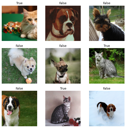

# train our model using resnet18 to keep it small and fast
learn = vision_learner(dls, resnet18, metrics = error_rate)
learn.fine_tune(3)

/usr/local/lib/python3.9/dist-packages/torchvision/models/_utils.py:208: UserWarning: The parameter 'pretrained' is deprecated since 0.13 and will be removed in 0.15, please use 'weights' instead.
  warnings.warn(
/usr/local/lib/python3.9/dist-packages/torchvision/models/_utils.py:223: UserWarning: Arguments other than a weight enum or `None` for 'weights' are deprecated since 0.13 and will be removed in 0.15. The current behavior is equivalent to passing `weights=ResNet18_Weights.IMAGENET1K_V1`. You can also use `weights=ResNet18_Weights.DEFAULT` to get the most up-to-date weights.
  warnings.warn(msg)
Downloading: "https://download.pytorch.org/models/resnet18-f37072fd.pth" to /root/.cache/torch/hub/checkpoints/resnet18-f37072fd.pth

epoch	train_loss	valid_loss	error_rate	time
0	0.199976	0.072374	0.020298	00:19

epoch	train_loss	valid_loss	error_rate	time
0	0.061802	0.081512	0.020974	00:20
1	0.047748	0.030506	0.010149	00:18
2	0.021600	0.026245	0.006766	00:18

# export our trained learner
learn.export('model.pkl')

Following the script in the video, as well as the git-lfs and requirements.txt in Tanishq Abraham’s tutorial, I deployed a Dog and Cat Classifier on HuggingFace Spaces.
If you run the training for long enough (high number of epochs) the error rate will get worse. We’ll learn why in a future lesson.
Use fastsetup to setup your local machine with Python and Jupyter.
- They recommend using mamba instead of conda as it is faster.

Notebook Exercise

In the cells below, I’ll run the code provided in the Chapter 2 notebook.

# prepare path and subfolder names
bear_types = 'grizzly', 'black', 'teddy'
path = Path('bears')

# download images of grizzly, black and teddy bears
if not path.exists():
    path.mkdir()
    for o in bear_types:
        dest = (path/o)
        dest.mkdir(exist_ok = True)
        results = search_images_ddg(f'{o} bear')
        download_images(dest, urls = results)

# view file paths
fns = get_image_files(path)
fns

(#570) [Path('bears/grizzly/ca9c20c9-e7f4-4383-b063-d00f5b3995b2.jpg'),Path('bears/grizzly/226bc60a-8e2e-4a18-8680-6b79989a8100.jpg'),Path('bears/grizzly/2e68f914-0924-42ed-9e2e-19963fa03a37.jpg'),Path('bears/grizzly/38e2d057-3eb2-4e8e-8e8c-fa409052aaad.jpg'),Path('bears/grizzly/6abc4bc4-2e88-4e28-8ce4-d2cbdb05d7b5.jpg'),Path('bears/grizzly/3c44bb93-2ac5-40a3-a023-ce85d2286846.jpg'),Path('bears/grizzly/2c7b3f99-4c8e-4feb-9342-dacdccf60509.jpg'),Path('bears/grizzly/a59f16a6-fa06-42d5-9d79-b84e130aa4e3.jpg'),Path('bears/grizzly/d1be6dc8-da42-4bee-ac31-0976b175f1e3.jpg'),Path('bears/grizzly/7bc0d3bd-a8dd-477a-aa16-449124a1afb5.jpg')...]

# get list of corrupted images
failed = verify_images(fns)
failed

(#24) [Path('bears/grizzly/2e68f914-0924-42ed-9e2e-19963fa03a37.jpg'),Path('bears/grizzly/f77cfeb5-bfd2-4c39-ba36-621f117a65f6.jpg'),Path('bears/grizzly/37aa7eed-5a83-489d-b8f5-54020ba41390.jpg'),Path('bears/black/90a464ad-b0a7-4cf5-86ff-72d507857007.jpg'),Path('bears/black/f03a0ceb-4983-4b8f-a001-84a0875704e8.jpg'),Path('bears/black/6193c1cf-fda4-43f9-844e-7ba7efd33044.jpg'),Path('bears/teddy/474bdbb3-de2f-49e5-8c5b-62b4f3f50548.JPG'),Path('bears/teddy/58755f3f-227f-4fad-badc-a7d644e54296.JPG'),Path('bears/teddy/eb55dc00-3d01-4385-a7da-d81ac5211696.jpg'),Path('bears/teddy/97eadc96-dc4e-4b3f-8486-88352a3b2270.jpg')...]

# remove corrupted image files
failed.map(Path.unlink)

(#24) [None,None,None,None,None,None,None,None,None,None...]

# create DataBlockfor training
bears = DataBlock(
    blocks = (ImageBlock, CategoryBlock),
    get_items = get_image_files,
    splitter = RandomSplitter(valid_pct = 0.2, seed = 42),
    get_y = parent_label,
    item_tfms = Resize(128)
)

# create DataLoaders object
dls = bears.dataloaders(path)

# view training batch -- looks good!
dls.show_batch(max_n = 4, nrows = 1)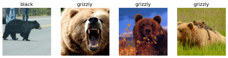

# view validation batch -- looks good!
dls.valid.show_batch(max_n = 4, nrows = 1)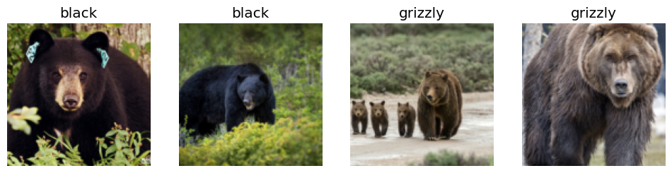

# observe how images react to the "squish" ResizeMethod
bears = bears.new(item_tfms = Resize(128, ResizeMethod.Squish))
dls = bears.dataloaders(path)
dls.valid.show_batch(max_n = 4, nrows = 1)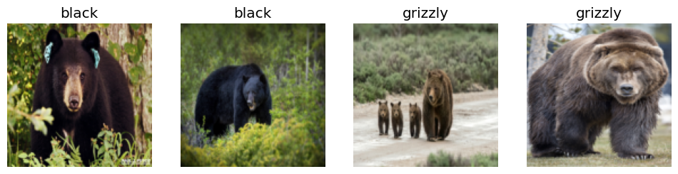

Notice how the grizzlies in the third image look abnormally skinny, since the image is squished.

# observe how images react to the "pad" ResizeMethod
bears = bears.new(item_tfms = Resize(128, ResizeMethod.Pad, pad_mode = 'zeros'))
dls = bears.dataloaders(path)
dls.valid.show_batch(max_n = 4, nrows = 1)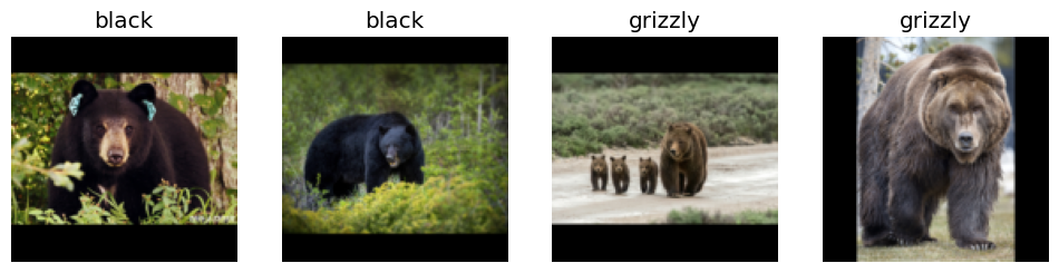

In these images, the original aspect ratio is maintained.

# observe how images react to the transform RandomResizedCrop
bears = bears.new(item_tfms = RandomResizedCrop(128, min_scale = 0.3))
dls = bears.dataloaders(path)
dls.valid.show_batch(max_n = 4, nrows = 1)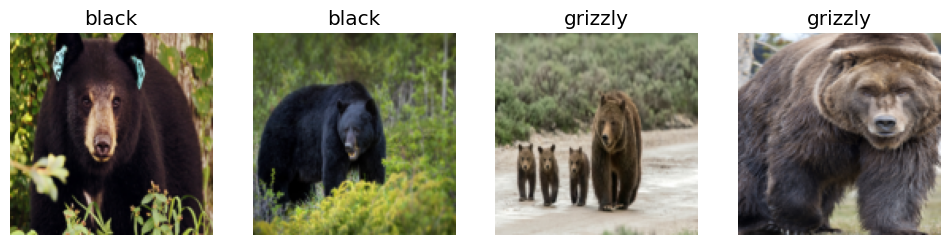

# observe how images react to data augmentation transforms
bears = bears.new(item_tfms=Resize(128), batch_tfms = aug_transforms(mult = 2))
dls = bears.dataloaders(path)
# note that data augmentation occurs on training set
dls.train.show_batch(max_n = 8, nrows = 2, unique = True)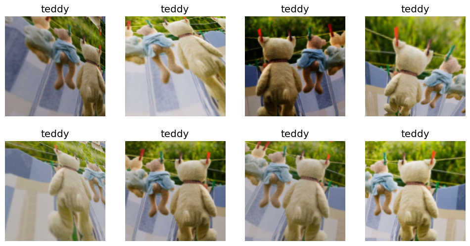

# train the model in order to clean the data
bears = bears.new(
    item_tfms = RandomResizedCrop(224, min_scale = 0.5),
    batch_tfms = aug_transforms())

dls = bears.dataloaders(path)
dls.show_batch()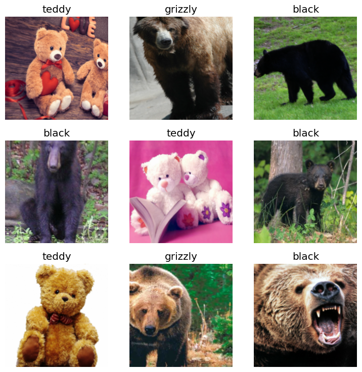

# train the model
learn = vision_learner(dls, resnet18, metrics = error_rate)
learn.fine_tune(4)

/usr/local/lib/python3.10/dist-packages/torchvision/models/_utils.py:208: UserWarning: The parameter 'pretrained' is deprecated since 0.13 and may be removed in the future, please use 'weights' instead.
  warnings.warn(
/usr/local/lib/python3.10/dist-packages/torchvision/models/_utils.py:223: UserWarning: Arguments other than a weight enum or `None` for 'weights' are deprecated since 0.13 and may be removed in the future. The current behavior is equivalent to passing `weights=ResNet18_Weights.IMAGENET1K_V1`. You can also use `weights=ResNet18_Weights.DEFAULT` to get the most up-to-date weights.
  warnings.warn(msg)
Downloading: "https://download.pytorch.org/models/resnet18-f37072fd.pth" to /root/.cache/torch/hub/checkpoints/resnet18-f37072fd.pth
100%|██████████| 44.7M/44.7M [00:00<00:00, 100MB/s]

epoch	train_loss	valid_loss	error_rate	time
0	1.221027	0.206999	0.055046	00:34

epoch	train_loss	valid_loss	error_rate	time
0	0.225023	0.177274	0.036697	00:32
1	0.162711	0.189059	0.036697	00:31
2	0.144491	0.191644	0.027523	00:31
3	0.122036	0.188296	0.018349	00:31

# view Confusion Matrix
interp = ClassificationInterpretation.from_learner(learn)
interp.plot_confusion_matrix()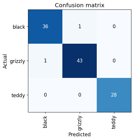

The model confused a grizzly for a black bear and a black bear for a grizzly bear. It didn’t confuse any of the teddy bears, which makes sense given how different they look to real bears.

# view images with the highest losses
interp.plot_top_losses(5, nrows = 1)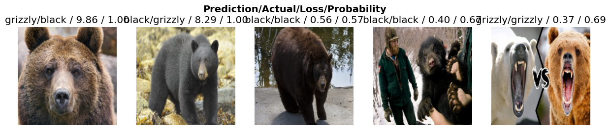

The fourth image has two humans in it, which is likely why the model didn’t recognize the bear. The model correctly predicted the the third and fifth images but with low confidence (57% and 69%).

# clean the training and validation sets
from fastai.vision.widgets import *

cleaner = ImageClassifierCleaner(learn)
cleaner

I cleaned up the images (deleting an image of a cat, another of a cartoon bear, a dog, and a blank image).

# delete or move images based on the dropdown selections made in the cleaner
for idx in cleaner.delete(): cleaner.fns[idx].unlink()
for idx,cat in cleaner.change(): shutil.move(str(cleaner.fns[idx]), path/cat)

# create new dataloaders object
bears = bears.new(
    item_tfms = RandomResizedCrop(224, min_scale = 0.5),
    batch_tfms = aug_transforms())

dls = bears.dataloaders(path)
dls.show_batch()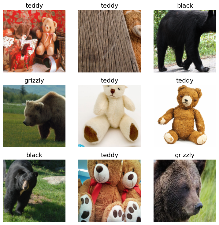

# retrain the model
learn = vision_learner(dls, resnet18, metrics = error_rate)
learn.fine_tune(4)

epoch	train_loss	valid_loss	error_rate	time
0	1.289331	0.243501	0.074074	00:32

epoch	train_loss	valid_loss	error_rate	time
0	0.225567	0.256021	0.064815	00:32
1	0.218850	0.288018	0.055556	00:34
2	0.184954	0.315183	0.055556	00:31
3	0.141363	0.308634	0.055556	00:31

Weird!! After cleaning the data, the model got worse (1.8% error rate is now 5.6%). I’ll run the cleaning routine again and retrain the model to see if it makes a difference. Perhaps there are still erroneous images in the mix.

# view Confusion Matrix
interp = ClassificationInterpretation.from_learner(learn)
interp.plot_confusion_matrix()

This time, the model incorrectly predicted 3 grizzlies as black bears, 2 black bears as grizzlies and 1 black bear as a teddy.

cleaner = ImageClassifierCleaner(learn)
cleaner

# delete or move images based on the dropdown selections made in the cleaner
for idx in cleaner.delete(): cleaner.fns[idx].unlink()
for idx,cat in cleaner.change(): shutil.move(str(cleaner.fns[idx]), path/cat)

# create new dataloaders object
bears = bears.new(
    item_tfms = RandomResizedCrop(224, min_scale = 0.5),
    batch_tfms = aug_transforms())

dls = bears.dataloaders(path)
# The lower right image (cartoon bear) is one that I selected "Delete" for
# in the cleaner so I'm not sure why it's still there
# I'm wondering if there's something wrong with the cleaner or how I'm using it?
dls.show_batch()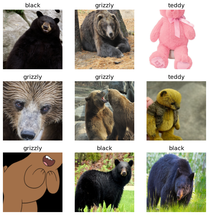

# retrain the model
learn = vision_learner(dls, resnet18, metrics = error_rate)
learn.fine_tune(4)

epoch	train_loss	valid_loss	error_rate	time
0	1.270627	0.130137	0.046729	00:31

epoch	train_loss	valid_loss	error_rate	time
0	0.183445	0.078030	0.028037	00:32
1	0.201080	0.053461	0.018692	00:33
2	0.183515	0.019479	0.009346	00:37
3	0.144900	0.012682	0.000000	00:31

I’m still not confident that this is a 100% accurate model given the bad images in the training set (such as the cartoon bear) but I’m going to go with it for now.

Book Notes

Chapter 2: From Model to Production

Underestimating the constraints and overestimating the capabilities of deep learning may lead to frustratingly poor results, at least until you gain some experience and can solve the problems that arise.
Overstimating the constraints and underestimating the capabilities of deep learning may mean you do not attempt a solvable problem because you talk yourself out of it.
The most important thing (as you learn deep learning) is to ensure that you have a project to work on.
The goal is not to find the “perfect” dataset or project, but just to get started and iterate from there.
Complete every step as well as you can in a reasonable amount of time, all the way to the end.
Computer vision
- Object recognition: recognize items in an image
- Object detection: recognition + highlight the location and name of each found object.
- Deep learning algorithms are generally not good at recognizing images that are significantly different in structure or style from those used to train the model.
NLP
- Deep learning is not good at generating correct responses.
- Text generation models will always be technologically a bit ahead of models for recognizing automatically generated text.
- Google’s online translation system is based on deep learning.
Combining text and images
- A deep learning model can be trained on input images with output captions written in English, and can learn to generate surprisingly appropriate captions automatically for new images (with no guarantee the captions will be correct).
- Deep learning should be used not as an entirely automated process, but as part of a process in which the model and a human user interact closely.
Tabular data
- If you already have a system that is using random forests or gradient boosting machines then switching to or adding deep learning may not result in any dramatic improvement.
- Deep learning greatly increases the variety of columns that you can include.
- Deep learning models generally take longer to train than random forests or gradient boosting machines.
Recommendation systems
- A special type of tabular data (a high-cardinality categorical variable representing users and another one representing products or something similar).
- Deep learning models are good at handling high cardinality categorical variables and thus recommendation systems.
- Deep learning models do well when combining these variables with other kinds of data such as natural language, images, or additional metadata represented as tables such as user information, previous transactions, and so forth.
- Nearly all machine learning approaches have th downside that they tell you only which products a particular user might like, rather than what recommendations would be helpful for a user.
Other data types
- Using NLP deep learning methods is the current SOTA approach for many types of protein analysis since protein chains look a lot like natural language documents.
The Drivetrain Approach
- Defined objective
- Levers (what inputs can we control)
- Data (what inputs we can collect)
- Models (how the levers influence the objective)
Gathering data
- For most projects you can find the data online.
- Use duckduckgo_search
From Data to DataLoaders
- DataLoaders is a thin class that just stores whatever DataLoader objects you pass to it and makes them available as train and valid.
- To turn data into a DataLoaders object we need to tell fastai four things:
  - What kinds of data we are working with.
  - How to get the list of items.
  - How to label these items.
  - How to create the validation set.
- With the DataBlock API you can customize every stage of the creation of your DataLoaders:

bears = DataBlock(
    blocks=(ImageBlock, CategoryBlock),
    get_items=get_image_files,
    splitter=RandomSplitter(valid_pct=0.2, seed=42),
    get_y=parent_label,
    item_tfms=Resize(128))

explanation of DataBlock
- blocks specifies types for independent (the thing we are using to make predictions from) and dependent (our target) variables.
- Computers don’t really know how to create random numbers at all, but simply create lists of numbers that look random; if you provide the same starting point for that list each time–called the seed–then you will get the exact same list each time.
- Images need to be all the same size.
- A DataLoader is a class that provides batches of a few items at a time to the GPU.
- fastai default batch size is 64 items.
- Resize crops the images to fit a square shape, alternatively you can pad (ResizeMethod.Pad) or squish (ResizeMethod.Squish) the images to fit the square.
- Squishing (model learns that things look differently from how they actually are), cropping (removal of features that would allow us to perform recognition) and padding (lot of empty space which is just wasted computation) are wasteful or problematic approaches. Instead, randomly select part of the image and then crop to just that part. On each epoch, we randomly select a different part of each image (RandomResizedCrop(min_scale)).
- Training the neural network with examples of images in which objects are in slightly different places and are slightly different sizes helps it to understand the basic concept of what an object is and how it can be represented in an image.
Data Augmentation
- refers to creating random variations of our input data, such that they appear different but do not change the meaning of the data (rotation, flipping, perspective warping, brightness changes, and contrast changes).
- aug_transforms() provides a standard set of augmentations.
- Use batch_tfms to process a batch at a time on the GPU to save time.
Training your model and using it to clean your data
- View confusion matrix with ClassificationInterpretation.from_learner(learn). The diagonal shows images that are classified correctly. Calculated using validation set.
- Sort images by loss using interp.plot_top_losses().
- Loss is high if the model is incorrect (especially if it’s also confident) or if it’s correct but not confident.
- A model can help you find data issues more quickly.
Using the model for inference
- learn.export() will export a .pkl file.
- Get predictions with learn_inf.predict(<input>). This returns three things: the predicted category in the same format you originally provided, the index of the predicted category and the probabilities for each category.
- You can access the DataLoaders as an attribute of the Learner: learn_inf.dls.
Deploying your app
- You almost certainly do not need a GPU to serve your model in production.
- To classify a few users’ images at a time, you need high-volume. If you do have this scenario, use Microsoft’s ONNX Runtime or AWS SageMaker.
- Recommended wherever possible to deploy the model itself to a server and have your mobile/edge application connect to it as a web service.
- If your application uses sensitive data, your users may be concerned about an approach that sends that data to a remote server.
How to Avoid Disaster
- Understanding and testing the behavior of a deep learning model is much more difficult than with most other code you write.
- The kinds of photos that people are most likely to upload to the internet are the kinds of photos that do a good job of clearly and artistically displaying their subject matter, which isn’t the kind of input this system is going to be getting in real life. We may need to do a lot of our own data collection and labeling to create a useful system.
- out-of-domain data: data that our model sees in production that is very different from what it saw during training.
- domain shift: data that our model sees changes over time.
- Deployment process
  - Manual Process: run model in parallel, humans check all predictions.
  - Limited scope deployment: careful human supervision, time or geography limited.
  - Gradual expansion: good reporting systems needed, consider what could go wrong.
- Unforeseen consequences and feedback loops
  - Your model may change the behavior of the system it’s a part of.
  - feedback loops can result in negative implications of bias getting worse.
  - A helpful exercise prior to rolling out a significant machine learning system is to consider the question “What would happen if it went really, really well?”
Questionnaire
1. Where do text models currently have a major deficiency?
  - Providing correct or accurate information.
2. What are possible negative societal implications of text generation models?
  - The viral spread of misinformation, which can lead to real actions and harms.
3. In situations where a model might make mistakes, and those mistakes could be harmful, what is a god alternative to automating a process?
  - Run the model in parallel with a human checking its predictions.
4. What kind of tabular data is deep learning particularly good at?
  - High-cardinality categorical data.
5. What’s a key downside of directly using a deep learning model for recommendation systems?
  - It will only tell you which products a particular user might like, rather than what recommendations may be helpful for a user.
6. What are the steps of the Drivetrain Approach?
  - Define an objective
  - Determine what inputs (levers) you can control
  - Collect data
  - Create models (how the levers influence the objective)
7. How do the steps of the Drivetrain Approach map to a recommendation system?
  - Objective: drive additional sales due to recommendations.
  - Level: ranking of the recommendations.
  - Data: must be collectd to generate recommendations that will cause new sales.
  - Models: two for purchasing probabilities conditional on seeing or not seeing a recommendation, the difference between these two probabilities is a utility function for a given recommendation to a customer (low in cases when algorithm recommends a familiar book that the customer has already rejected, or a book they would have bought even without the recommendation).
8. Create an image recognition model using data you curate, and deploy it on the web.
  - Here.
9. What is DataLoaders?
  - A class that creates validation and training sets/batches that are fed to the GPUS
10. What four things do we need to tell fastai to create DataLoaders?
  - What kinds of data we are working with (independent and dependent variables).
  - How to get the list of items.
  - How to label these items.
  - How to create the validation set.
11. What does the splitter parameter to DataBlock do?
  - Set aside a percentage of the data as the validation set.
12. How do we ensure a random split always gives the same validation set?
  - Set the seed parameter to the same value.
13. What letters are often used to signify the independent and dependent variables?
  - Independent: x
  - Dependent: y
14. What’s the difference between crop, pad and squish resize approaches? When might you choose one over the others?
  - Crop: takes a section of the image and resizes it to the desired size. Use when it’s not necessary to have the model traing on the whole image.
  - Pad: keep the image aspect ratio as is, add white/black padding to make a square. Use when it’s necessary to have the model train on the whole image.
  - Squish: distorts the image to fit a square. Use when it’s not necessary to have the model train on the original aspect ratio.
15. What is data augmentation? Why is it needed?
  - Data augmentation is the creation of random variations of input data through techniques like rotation, flipping, brightness changes, contrast changes, perspective warping. It is needed to help the model learn to recognize objects under different lighting/perspective conditions.
16. Provide an example of where the bear classification model might work poorly in production, due to structural or style differences in the training data.
17. What is the difference between item_tfms and batch_tfms?
  - item_tfms are transforms that are applied to each item in the set.
  - batch_tfms are transforms applied to a batch of items in the set.
18. What is a confusion matrix?
  - A matrix that shows the counts of predicted (columns) vs. actual (rows) labels, with the diagonal being correctly predicted data.
19. What does export save?
  - Both the architecture and the parameters as a .pkl file.
20. What is called when we use a model for making predictions, instead of training?
  - Inference
21. What are IPython widgets?
  - interactive browser controls for Jupyter Notebooks.
22. When would you use a CPU for deployment? When might a GPU be better?
  - CPU: low-volume, single-user inputs for prediction.
  - GPU: high-volume, multiple-user inputs for predictions.
23. What are the downsides of deploying your app to a server, instead of to a client (or edge) device such as a phone or PC?
  - Requires internet connectivity (and latency).
  - Sensitive data transfer may not be okay with your users.
  - Managing complexity and scaling the server creates additional overhead.
24. What are three examples of problems that could occur when rolling out a bear warning system in practice?
  - out-of-domain data: the images captured of real bears may not be represented in the model’s training or validation datasets.
  - Number of bear alerts doubles or halves after rollout of the new system in some location.
  - out-of-domain data: the cameras may capture low-resolution images of the bears when the training and validation set had high resolution images.
25. What is out-of-domain data?
  - Data your model sees in production that it hasn’t seen during training.
26. What is domain shift?
  - Changes in the data that our model sees in production over time.
27. What are the three steps in the deployment process?
  - Manual Process
  - Limited scope deployment
  - Gradual expansion
Further Research
1. Consider how the Drivetrain Approach maps to a project or problem you’re interested in.
  - I’ll take the example of a project I will be working on to practice what I’m learning in this book: training a deep learning model which correctly classifies the typeface from a collection of single letter.
    - The objective: correctly classify typeface from a collection of single letters.
    - Levers: observe key features of key letters that are the “tell” of a typeface.
    - Data: using an HTML canvas object and Adobe Fonts, generate images of single letters of multiple fonts associated with each category of typeface.
    - Models: output the probabilities of each typeface a given collection of single letters is predicted as. This allows for some flexibility in how you categorize letters based on the shared characteristics of more than one typeface that the particular font may possess.
2. When might it be best to avoid certain types of data augmentation?
  - In my typeface example, it’s best to avoid perspective warping because it will change key features used to recognize a typeface.
3. For a project you’re interested in applying deep learning to, consider the thought experiment, “What would happen if it went really, really well?”
  - If my typeface classifier works really well, I imagine it would be used by people to take pictures of real-world text and learn what typeface it is. This may inspire a new wave of typeface designers. If a feedback loop was possible, and the classifier went viral, the very definition of typefaces may be affected by popular opinion. Taken a step further, a generative model may be inspired by this classifier, and a new wave of AI typeface would be launched—however this last piece is highly undesirable unless the training of the model involves appropriate licensing and attribution of the typefaces used that are created by humans. Furthermore, from what I understand from reading about typefaces, the process of creating a typeface is an amazing experience and should not be replaced with AI generators. If I created such a generative model (in part 2 of the course) and it went viral (do HuggingFace Spaces go viral? Cuz that’s where I would launch it), I would take it down.
4. Start a blog (done!)

Lesson 3: Neural Net Foundations

Video Notes

Link to this lesson’s video.

How to do a fast.ai lesson
- Watch lecture
- Run notebook & experiment
- Reproduce results
- Repeat with different dataset
fastbook repo contains “clean” folder with notebooks without markdown text.
Two concepts: training the model and using it for inference.
Over 500 architectures in timm (PyTorch Image Models).
timm.list_models(pattern) will list models matching the pattern.
Pass string name of timm model to the Learner like: vision_learner(dls, 'timm model string', ...).
in22 = ImageNet with 22k categories, 1k = ImageNet with 1k categories.
learn.predict probabilities are in the order of learn.dls.vocab.
learn.model contains the trained model which contains lots of nested layers.
learn.model.get_submodule takes a dotted string navigating through the hierarchy.
Machine learning models fit functions to data.
Things between dollar signs is LaTeX "$...$".
General form of quadratic: def quad(a,b,c,x): return a*x**2 + b*x + c
partial from functools fixes parameters to a function.
Loss functions tells us how good our model is.
@interact from ipywidgets allows sliders tied to the function its above.
Mean Squared Error: def mse(preds, acts): return ((preds - acts)**2).mean()
For each parameter we need to know: does the loss get better when we increase or decrease the parameter?
The derivative is the function that tells you: if you increase the input does the output increase or decrease, and by how much?
*params spreads out the list into its elements and passes each to the function.
1-D (rank 1) tensor (lists of numbers), 2-D tensor (tables of numbers) 3-D tensor (layers of tables of numbers) and so on.
tensor.requires_grad_() calculates the gradient of the values in the tensor whenever its used in calculation.
loss.backward() calculates gradients on the inputs to the loss function.
abc.grad attribute added after gradients are calculated.
negative gradient means increasing the parameter will decrease the loss.
update parameters with torch.no_grad() so PyTorch doesn’t calculate the gradient (since it’s being used in a function). We don’t want the derivative of the parameter update, we only want the derivative with respect to the loss.
Automate the steps
- Calculate Mean Squared Error
- Call .backward.
- Subtract gradient * small number from the parameters
All optimizers are built on the concept of gradient descent (calculate gradients and decrease the loss).
We need a better function than quadratics
Rectified Linear Unit:

def rectified_linear(m,b,x):
    y = m*x + b
    return torch.clip(y, 0.)

torch.clip turns values less than value specified to the value specified (in this case, it turns negative values to 0.).
Adding rectified linear functions together gives us an arbitrarily squiggly function that will match as close as we want to the data.
ReLU in 2D gives you surfaces, volumes in 3D, etc.
With this incredibly simple foundation you can construct an arbitrarily precise, accurate model.
When you have ReLU’s getting added together, and gradient descent to optimize the parameters, and samples of inputs and outputs that you want, the computer “draws the owl” so to speak.
Deep learning is using gradient descent to set some parameters to make a wiggly function (the addition of lots of rectified linear units or something very similar to that) that matches your data.
When selecting an architecture, the biggest beginner mistake is that they jump to the highest-accuracy models.
At the start of the project, just use resnet18 so you can spend all of your time trying things out (data augmentation, data cleaning, different external data) as fast as possible.
Trying better architectures is the very last thing to do.
How do I know if I have enough data?
- Vast majority of projects in industry wait far too long until they train their first model.
- Train your first model on day 1 with whatever CSV files you can hack together.
- Semi-supervised training lets you get dramatically more out of your data.
- Often it’s easy to get lots of inputs but hard to get lots of outputs (labels).
Units of parameter gradients: for each increase in parameter of 1, the gradient is the amount the loss would change by (if it stayed at that slope—which it doesn’t because it’s a curve).
Once you get close enough to the optimal parameter value, all loss functions look like quadratics
- The slope of the loss function decreases as you approach the optimal
Learning rate (a hyperparameter) is multiplied by the gradient, the product of which is subtracted from the parameters
If you pick a learning rate that’s too large, you will diverge; if you pick too small, it’ll take too long to train.
http://matrixmultiplication.xyz/
Matrix multiplication is the critical foundational mathematical operation in deep learning
GPUs are good at matrix multiplication with tensor cores (multiply together two 4x4 matrices)
Use a spreadsheet to train a deep learning model on the Kaggle Titanic dataset in which you’re trying to predict if a person survived.
- Columns included (convert some of them to binary categorical variables):
  - Survivor
  - Pclass
    - Convert to Pclass_1 and Pclass_2 (both 1/0).
  - Sex
    - Convert to Male (0/1) column.
  - Age
    - Remove blanks.
    - Normalize (Age/Max(Age))
  - SibSp (how many siblings they have)
  - Parch (# of parents/children aboard)
  - Fare
    - Lots of very small and very large fares, log of it has a much more even distribution. (LOG10(Fare + 1).
  - Embarked (which city they got on at)
    - Remove blanks.
    - Convert to Embark_S and Embark_C (both 1/0)
  - Ones
    - Add a column of 1s.
- Create random numbers for params (including Const) with =RAND() - 0.5.
- Regression
  - Use SUMPRODUCT to calculate linear function.
  - Loss of linear function is (linear function result - Survived) ^ 2.
  - Average loss = AVERAGE(individual losses).
  - User “Solver” with GRG Nonlinear Solving Method. Set Objective to minimize the cell with average loss. Change parameter variables.
- Neural Net
  - Two sets of params.
  - Two linear columns.
  - Two ReLU columns.
  - Adding two linear functions together gives you a linear function, we want all those wiggles (non-linearity) so we use ReLUs.
  - ReLU: IF(lin1 < 0, 0, lin1)
  - Preds = sum of the two ReLUs.
  - Loss same as regression.
  - Solver process the same as well.
- Neural Net (Matrix Multiplication)
  - Transpose params into two columns.
  - =MMULT(...) for Lin1 and Lin2 columns.
  - Keep ReLU, Preds and Loss column the same.
  - Optimize params using Solver.
  - Helpful reminder to build intuition around matrix multiplication: it’s doing the same thing as the SUMPRODUCTs.
- Dummy variables: Pclass_1, Pclass_2, etc.
Next lesson: NLP
- It’s about making predictions with text data which most of the time is in the form of prose.
- First Farsi NLP resource was created by a student of the first fastai course.
- NLP most commonly and practically used for classification.
- Document = one or two words, a book, a wikipedia page, any length.
- Classification = figure out a category for a document.
- Sentiment analysis
- Author identification
- Legal discovery (is this document in-scope or out-of-scope)
- Organizing documents by topic
- Triaging inbound emails
- Classification of text looks similar to images.
- We’re going to use a different library: HuggingFace Transformers
  - Helpful to see how things are done in more than one library.
  - HuggingFace Transformers doesn’t have the same high-level API. Have to do more stuff manually. Which is good for students at this point of the course.
  - It’s a good library.
- Before the next lesson take a look at the NLP notebook and U.S. Patent to Phrase Matching data.
  - Trying to figure out in patents whether two concepts are referring to the same thing. The document is text1, text2, and the category is similar (1) or not-similar (0).
- Will also talk about the two very important topics of validation sets and metrics.

Notebook Exercise

Training and Deploying: Pets Classifier

In this section, I’ll train a Pets dataset classifier as done by Jeremy in this notebook.

from fastai.vision.all import *
import timm

path = untar_data(URLs.PETS)/'images'

# Create DataLoaders object
dls = ImageDataLoaders.from_name_func('.',
                                      get_image_files(path),
                                      valid_pct=0.2,
                                      seed=42,
                                      label_func=RegexLabeller(pat = r'^([^/]+)_\d+'),
                                      item_tfms=Resize(224))

100.00% [811712512/811706944 01:00<00:00]

dls.show_batch(max_n=4)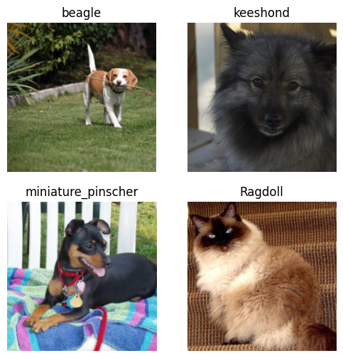

# train using resnet34 as architecture
learn = vision_learner(dls, resnet34, metrics=error_rate)
learn.fine_tune(3)

/usr/local/lib/python3.10/dist-packages/torchvision/models/_utils.py:208: UserWarning: The parameter 'pretrained' is deprecated since 0.13 and may be removed in the future, please use 'weights' instead.
  warnings.warn(
/usr/local/lib/python3.10/dist-packages/torchvision/models/_utils.py:223: UserWarning: Arguments other than a weight enum or `None` for 'weights' are deprecated since 0.13 and may be removed in the future. The current behavior is equivalent to passing `weights=ResNet34_Weights.IMAGENET1K_V1`. You can also use `weights=ResNet34_Weights.DEFAULT` to get the most up-to-date weights.
  warnings.warn(msg)
Downloading: "https://download.pytorch.org/models/resnet34-b627a593.pth" to /root/.cache/torch/hub/checkpoints/resnet34-b627a593.pth
100%|██████████| 83.3M/83.3M [00:00<00:00, 196MB/s]

epoch	train_loss	valid_loss	error_rate	time
0	1.496086	0.316146	0.100135	01:12

0.00% [0/3 00:00<?]

epoch	train_loss	valid_loss	error_rate	time

45.65% [42/92 00:25<00:30 0.4159]

epoch	train_loss	valid_loss	error_rate	time
0	0.441153	0.315289	0.093369	01:04
1	0.289844	0.215224	0.069012	01:05
2	0.123374	0.191152	0.060217	01:03

The pets classifier, using resnet34 and 3 epochs, is about 94% accurate.

# train using a timm architecture
# from the convnext family of architectures
learn = vision_learner(dls, 'convnext_tiny_in22k', metrics=error_rate).to_fp16()
learn.fine_tune(3)

/usr/local/lib/python3.10/dist-packages/timm/models/_factory.py:114: UserWarning: Mapping deprecated model name convnext_tiny_in22k to current convnext_tiny.fb_in22k.
  model = create_fn(

epoch	train_loss	valid_loss	error_rate	time
0	1.130913	0.240275	0.085927	01:06

epoch	train_loss	valid_loss	error_rate	time
0	0.277886	0.193888	0.061570	01:08
1	0.196232	0.174544	0.055480	01:09
2	0.127525	0.156720	0.048038	01:07

Using convnext_tiny_in22k, the model is about 95.2% accurate, about a 20% decrease in error rate.

# export to use in gradio app
learn.export('pets_model.pkl')

You can view my pets classifier gradio app here.

Which image models are best?

In this section, I’ll plot the timm model results as shown in Jeremy’s notebook.

import pandas as pd

# load data
df_results = pd.read_csv("../../../fastai-course/data/results-imagenet.csv")
df_results.head()

	model	top1	top1_err	top5	top5_err	param_count	img_size	crop_pct	interpolation
0	eva02_large_patch14_448.mim_m38m_ft_in22k_in1k	90.052	9.948	99.048	0.952	305.08	448	1.0	bicubic
1	eva02_large_patch14_448.mim_in22k_ft_in22k_in1k	89.966	10.034	99.012	0.988	305.08	448	1.0	bicubic
2	eva_giant_patch14_560.m30m_ft_in22k_in1k	89.786	10.214	98.992	1.008	1,014.45	560	1.0	bicubic
3	eva02_large_patch14_448.mim_in22k_ft_in1k	89.624	10.376	98.950	1.050	305.08	448	1.0	bicubic
4	eva02_large_patch14_448.mim_m38m_ft_in1k	89.570	10.430	98.922	1.078	305.08	448	1.0	bicubic

top1 = what percent of the time the model predicts the correct label with the highest probability.

top5 = what percent of the time the model predits the correct label with the top 5 highest probabilities.

Source

# remove additional text from model name
df_results['model_org'] = df_results['model']
df_results['model'] = df_results['model'].str.split('.').str[0]
df_results.head()

	model	top1	top1_err	top5	top5_err	param_count	img_size	crop_pct	interpolation	model_org
0	eva02_large_patch14_448	90.052	9.948	99.048	0.952	305.08	448	1.0	bicubic	eva02_large_patch14_448.mim_m38m_ft_in22k_in1k
1	eva02_large_patch14_448	89.966	10.034	99.012	0.988	305.08	448	1.0	bicubic	eva02_large_patch14_448.mim_in22k_ft_in22k_in1k
2	eva_giant_patch14_560	89.786	10.214	98.992	1.008	1,014.45	560	1.0	bicubic	eva_giant_patch14_560.m30m_ft_in22k_in1k
3	eva02_large_patch14_448	89.624	10.376	98.950	1.050	305.08	448	1.0	bicubic	eva02_large_patch14_448.mim_in22k_ft_in1k
4	eva02_large_patch14_448	89.570	10.430	98.922	1.078	305.08	448	1.0	bicubic	eva02_large_patch14_448.mim_m38m_ft_in1k

def get_data(part, col):
    # get benchmark data and merge with model data
    df = pd.read_csv(f'../../../fastai-course/data/benchmark-{part}-amp-nhwc-pt111-cu113-rtx3090.csv').merge(df_results, on='model')
    # convert samples/sec to sec/sample
    df['secs'] = 1. / df[col]
    # pull out the family name from the model name
    df['family'] = df.model.str.extract('^([a-z]+?(?:v2)?)(?:\d|_|$)')
    # removing `resnetv2_50d_gn` and `resnet50_gn` for some reason
    df = df[~df.model.str.endswith('gn')]
    # not sure why the following line is here, "in22" was removed in cell above
    df.loc[df.model.str.contains('in22'),'family'] = df.loc[df.model.str.contains('in22'),'family'] + '_in22'
    df.loc[df.model.str.contains('resnet.*d'),'family'] = df.loc[df.model.str.contains('resnet.*d'),'family'] + 'd'
    # only returns subset of families
    return df[df.family.str.contains('^re[sg]netd?|beit|convnext|levit|efficient|vit|vgg|swin')]

# load benchmark inference data
df = get_data('infer', 'infer_samples_per_sec')
df.head()

	model	infer_samples_per_sec	infer_step_time	infer_batch_size	infer_img_size	param_count_x	top1	top1_err	top5	top5_err	param_count_y	img_size	crop_pct	interpolation	model_org	secs	family
12	levit_128s	21485.80	47.648	1024	224	7.78	76.526	23.474	92.872	7.128	7.78	224	0.900	bicubic	levit_128s.fb_dist_in1k	0.000047	levit
13	regnetx_002	17821.98	57.446	1024	224	2.68	68.746	31.254	88.536	11.464	2.68	224	0.875	bicubic	regnetx_002.pycls_in1k	0.000056	regnetx
15	regnety_002	16673.08	61.405	1024	224	3.16	70.278	29.722	89.528	10.472	3.16	224	0.875	bicubic	regnety_002.pycls_in1k	0.000060	regnety
17	levit_128	14657.83	69.849	1024	224	9.21	78.490	21.510	94.012	5.988	9.21	224	0.900	bicubic	levit_128.fb_dist_in1k	0.000068	levit
18	regnetx_004	14440.03	70.903	1024	224	5.16	72.398	27.602	90.828	9.172	5.16	224	0.875	bicubic	regnetx_004.pycls_in1k	0.000069	regnetx

# plot the data
import plotly.express as px
w,h = 1000, 800

def show_all(df, title, size):
    return px.scatter(df,
                      width=w,
                      height=h,
                      size=df[size]**2,
                      title=title,
                      x='secs',
                      y='top1',
                      log_x=True,
                      color='family',
                      hover_name='model_org',
                      hover_data=[size]
                     )

show_all(df, 'Inference', 'infer_img_size')

# plot a subset of the data
subs = 'levit|resnetd?|regnetx|vgg|convnext.*|efficientnetv2|beit|swin'

def show_subs(df, title, size, subs):
    df_subs = df[df.family.str.fullmatch(subs)]
    return px.scatter(df_subs,
                      width=w,
                      height=h,
                      size=df_subs[size]**2,
                      title=title,
                      trendline='ols',
                      trendline_options={'log_x':True},
                      x='secs',
                      y='top1',
                      log_x=True,
                      color='family',
                      hover_name='model_org',
                      hover_data=[size])

show_subs(df, 'Inference', 'infer_img_size', subs)

# plot inference speed vs parameter count
px.scatter(df,
           width=w,
           height=h,
           x='param_count_x',
           y='secs',
           log_x=True,
           log_y=True,
           color='infer_img_size',
           hover_name='model_org',
           hover_data=['infer_samples_per_sec', 'family']
)

# repeat plots for training data
tdf = get_data('train', 'train_samples_per_sec')
show_all(tdf, 'Training', 'train_img_size')

# subset of training data
show_subs(tdf, 'Training', 'train_img_size', subs)

How does a neural net really work?

In this section, I’ll recreate the content in Jeremy’s notebook here, where he walks through a quadratic example of training a function to match the data.

A neural network layer:

Multiplies each input by a number of values. These values are known as parameters.
Adds them up for each group of values.
Replaces the negative numbers with zeros.

# helper functions
from ipywidgets import interact
from fastai.basics import *

# helper functions
plt.rc('figure', dpi=90)

def plot_function(f, title=None, min=-2.1, max=2.1, color='r', ylim=None):
    x = torch.linspace(min,max, 100)[:,None]
    if ylim: plt.ylim(ylim)
    plt.plot(x, f(x), color)
    if title is not None: plt.title(title)

In the plot_function definition, I’ll look into why [:,None] is added after torch.linspace(min, max, 100)

torch.linspace(-1, 1, 10), torch.linspace(-1, 1, 10).shape

(tensor([-1.0000, -0.7778, -0.5556, -0.3333, -0.1111,  0.1111,  0.3333,  0.5556,
          0.7778,  1.0000]),
 torch.Size([10]))

torch.linspace(-1, 1, 10)[:,None], torch.linspace(-1, 1, 10)[:,None].shape

(tensor([[-1.0000],
         [-0.7778],
         [-0.5556],
         [-0.3333],
         [-0.1111],
         [ 0.1111],
         [ 0.3333],
         [ 0.5556],
         [ 0.7778],
         [ 1.0000]]),
 torch.Size([10, 1]))

[:, None] adds a dimension to the tensor.

Next he fits a quadratic function to data:

def f(x): return 3*x**2 + 2*x + 1

plot_function(f, '$3x^2 + 2x + 1$')

In order to simulate “finding” or “learning” the right model fit, he creates a general quadratic function:

def quad(a, b, c, x): return a*x**2 + b*x + c

and uses partial to make new quadratic functions:

def mk_quad(a, b, c): return partial(quad, a, b, c)

# recreating original quadratic with mk_quad
f2 = mk_quad(3, 2, 1)
plot_function(f2)

f2

functools.partial(<function quad at 0x148c6d000>, 3, 2, 1)

quad

<function __main__.quad(a, b, c, x)>

Next he simulates noisy measurements of the quadratic f:

# `scale` parameter is the standard deviation of the distribution
def noise(x, scale): return np.random.normal(scale=scale, size=x.shape)

# noise function matches quadratic x + x^2 (with noise) + constant noise
def add_noise(x, mult, add): return x * (1+noise(x, mult)) + noise(x,add)

np.random.seed(42)

x = torch.linspace(-2, 2, steps=20)[:, None]
y = add_noise(f(x), 0.15, 1.5)

# values match Jeremy's
x[:5], y[:5]

(tensor([[-2.0000],
         [-1.7895],
         [-1.5789],
         [-1.3684],
         [-1.1579]]),
 tensor([[11.8690],
         [ 6.5433],
         [ 5.9396],
         [ 2.6304],
         [ 1.7947]], dtype=torch.float64))

plt.scatter(x, y)

# overlay data with variable quadratic
@interact(a=1.1, b=1.1, c=1.1)
def plot_quad(a, b, c):
    plt.scatter(x, y)
    plot_function(mk_quad(a, b, c), ylim=(-3,13))

Important note changing sliders: only after changing b and c values do you realize that a also needs to be changed.

Next, he creates a measure for how well the quadratic fits the data, mean absolute error (distance from each data point to the curve).

def mae(preds, acts): return (torch.abs(preds-acts)).mean()

# update interactive plot
@interact(a=1.1, b=1.1, c=1.1)
def plot_quad(a, b, c):
    f = mk_quad(a,b,c)
    plt.scatter(x,y)
    loss = mae(f(x), y)
    plot_function(f, ylim=(-3,12), title=f"MAE: {loss:.2f}")

In a neural network we’ll have tens of millions or more parameters to fit and thousands or millions of data points to fit them to, which we can’t do manually with sliders. We need to automate this process.

If we know the gradient of our mae() function with respect to our parameters, a, b and c, then that means we know how adjusting a parameter will change the function. If, say, a has a negative gradient, then we know increasing a will decrease mae(). So we find the gradient of the parameters with respect to the loss function and adjust our parameters a bit in the opposite direction of the gradient sign.

To do this we need a function that will take the parameters as a single vector:

def quad_mae(params):
    f = mk_quad(*params)
    return mae(f(x), y)

# testing it out
# should equal 2.4219
quad_mae([1.1, 1.1, 1.1])

tensor(2.4219, dtype=torch.float64)

# pick an arbitrary starting point for our parameters
abc = torch.tensor([1.1, 1.1, 1.1])

# tell pytorch to calculate its gradients
abc.requires_grad_()

# calculate loss
loss = quad_mae(abc)
loss

tensor(2.4219, dtype=torch.float64, grad_fn=<MeanBackward0>)

# calculate gradients
loss.backward()

# view gradients
abc.grad

tensor([-1.3529, -0.0316, -0.5000])

# increase parameters to decrease loss based on gradient sign
with torch.no_grad():
    abc -= abc.grad*0.01
    loss = quad_mae(abc)

print(f'loss={loss:.2f}')

loss=2.40

The loss has gone down from 2.4219 to 2.40. We’re moving in the right direction.

The small number we multiply gradients by is called the learning rate and is the most important hyper-parameter to set when training a neural network.

# use a loop to do a few more iterations
for i in range(10):
    loss = quad_mae(abc)
    loss.backward()
    with torch.no_grad(): abc -= abc.grad*0.01
    print(f'step={i}; loss={loss:.2f}')

step=0; loss=2.40
step=1; loss=2.36
step=2; loss=2.30
step=3; loss=2.21
step=4; loss=2.11
step=5; loss=1.98
step=6; loss=1.85
step=7; loss=1.72
step=8; loss=1.58
step=9; loss=1.46

The loss continues to decrease. Here are our parameters and their gradients at this stage:

abc

tensor([1.9634, 1.1381, 1.4100], requires_grad=True)

abc.grad

tensor([-13.4260,  -1.0842,  -4.5000])

A neural network can approximate any computable function, given enough parameters using two key steps:

Matrix multiplication.
The function $max(x,0)$, which simply replaces all negative numbers with zero.

The combination of a linear function and $max$ is called a rectified linear unit and can be written as:

def rectified_linear(m,b,x):
    y = m*x+b
    return torch.clip(y, 0.)

plot_function(partial(rectified_linear, 1, 1))

# we can do the same thing using PyTorch
import torch.nn.functional as F
def rectified_linear2(m,b,x): return F.relu(m*x+b)
plot_function(partial(rectified_linear2, 1,1))

Create an interactive ReLU:

@interact(m=1.5, b=1.5)
def plot_relu(m, b):
    plot_function(partial(rectified_linear, m, b), ylim=(-1,4))

Observe what happens when we add two ReLUs together:

def double_relu(m1,b1,m2,b2,x):
    return rectified_linear(m1,b1,x) + rectified_linear(m2,b2,x)

@interact(m1=-1.5, b1=-1.5, m2=1.5, b2=1.5)
def plot_double_relu(m1, b1, m2, b2):
    plot_function(partial(double_relu, m1,b1,m2,b2), ylim=(-1,6))

Creating a triple ReLU function to fit our data:

def triple_relu(m1,b1,m2,b2,m3,b3,x):
    return rectified_linear(m1,b1,x) + rectified_linear(m2,b2,x) + rectified_linear(m3,b3,x)

def mk_triple_relu(m1,b1,m2,b2,m3,b3): return partial(triple_relu, m1,b1,m2,b2,m3,b3)

@interact(m1=-1.5, b1=-1.5, m2=0.5, b2=0.5, m3=1.5, b3=1.5)
def plot_double_relu(m1, b1, m2, b2, m3, b3):
    f = mk_triple_relu(m1,b1,m2,b2,m3,b3)
    plt.scatter(x,y)
    loss = mae(f(x), y)
    plot_function(f, ylim=(-3,12), title=f"MAE: {loss:.2f}")

This same approach can be extended to functions with 2, 3, or more parameters. Drawing squiggly lines through some points is literally all that deep learning does. The above steps will, given enough time and enough data, create (for example) an owl recognizer if you feed it enough owls and non-owls.

We can could do thousands of computations on a GPU instead of the above CPU computation. We can greatly reduce the amount of computation and data needed by using a convolution instead of a matrix multiplication. We could make things much faster if, instead of starting with random parameters, we start with parameters of someone else’s model that does something similar to what we want (transfer learning).

Gradient Descent with Microsoft Excel

Following the instructions in the fastai course lesson video, I’ve created a Microsoft Excel deep learning model here for the Titanic Kaggle data.

As shown in the course video, I trained three different models—linear regression, neural net (using SUMPRODUCT) and neural net (using MMULT). After running Microsoft Excel’s Solver, I got the final (different than video) mean loss for each model:

linear: 0.14422715
nnet: 0.14385956
mmult: 0.14385956

The linear model loss in the video was about 0.10 and the neural net loss was about 0.08. So, my models didn’t do as well.

Book Notes

In this section, I’ll take notes while reading Chapter 4 in the fastai textbook.

Pixels: The Foundations of Computer Vision

We’ll use the MNIST dataset for our experiments, which contains handwritten digits.
MNIST is collected by the National Institute of Standards and Technology and collated into a machine learning dataset by Yann Lecun who used MNIST in 1998 in LeNet-5, the first computer system to demonstrate practically useful recognition of handwritten digits.
We’ve seen that the only consisten trait among every fast.ai student who’s gone on to be a world-class practitioner is that they are all very tenacious.
In this chapter we’ll create a model that can classify any image as a 3 or a 7.

from fastai.vision.all import *

path = untar_data(URLs.MNIST_SAMPLE)

100.14% [3219456/3214948 00:00<00:00]

# ls method added by fastai
# lists the count of items
path.ls()

(#3) [Path('/root/.fastai/data/mnist_sample/labels.csv'),Path('/root/.fastai/data/mnist_sample/train'),Path('/root/.fastai/data/mnist_sample/valid')]

(path/'train').ls()

(#2) [Path('/root/.fastai/data/mnist_sample/train/3'),Path('/root/.fastai/data/mnist_sample/train/7')]

# 3 and 7 are the labels
threes = (path/'train'/'3').ls().sorted()
sevens = (path/'train'/'7').ls().sorted()
threes

(#6131) [Path('/root/.fastai/data/mnist_sample/train/3/10.png'),Path('/root/.fastai/data/mnist_sample/train/3/10000.png'),Path('/root/.fastai/data/mnist_sample/train/3/10011.png'),Path('/root/.fastai/data/mnist_sample/train/3/10031.png'),Path('/root/.fastai/data/mnist_sample/train/3/10034.png'),Path('/root/.fastai/data/mnist_sample/train/3/10042.png'),Path('/root/.fastai/data/mnist_sample/train/3/10052.png'),Path('/root/.fastai/data/mnist_sample/train/3/1007.png'),Path('/root/.fastai/data/mnist_sample/train/3/10074.png'),Path('/root/.fastai/data/mnist_sample/train/3/10091.png')...]

# view one of the images
im3_path = threes[1]
im3 = Image.open(im3_path)
im3

# the image is stored as numbers
array(im3)[4:10, 4:10]

array([[  0,   0,   0,   0,   0,   0],
       [  0,   0,   0,   0,   0,  29],
       [  0,   0,   0,  48, 166, 224],
       [  0,  93, 244, 249, 253, 187],
       [  0, 107, 253, 253, 230,  48],
       [  0,   3,  20,  20,  15,   0]], dtype=uint8)

# same thing, but a PyTorch tensor
tensor(im3)[4:10, 4:10]

tensor([[  0,   0,   0,   0,   0,   0],
        [  0,   0,   0,   0,   0,  29],
        [  0,   0,   0,  48, 166, 224],
        [  0,  93, 244, 249, 253, 187],
        [  0, 107, 253, 253, 230,  48],
        [  0,   3,  20,  20,  15,   0]], dtype=torch.uint8)

# use pandas.DataFrame to color code the array
im3_t = tensor(im3)
df = pd.DataFrame(im3_t[4:15, 4:22])
df.style.set_properties(**{'font-size': '6pt'}).background_gradient('Greys')

	1	2	3	4	5	6	7	8	9	10	11	12	13	14	15	16
0	0	0	0	0	0	0	0	0	0	0	0	0	0	0	0	0
1	0	0	0	0	29	150	195	254	255	254	176	193	150	96	0	0
2	0	0	48	166	224	253	253	234	196	253	253	253	253	233	0	0
3	93	244	249	253	187	46	10	8	4	10	194	253	253	233	0	0
4	107	253	253	230	48	0	0	0	0	0	192	253	253	156	0	0
5	3	20	20	15	0	0	0	0	0	43	224	253	245	74	0	0
6	0	0	0	0	0	0	0	0	0	249	253	245	126	0	0	0
7	0	0	0	0	0	0	14	101	223	253	248	124	0	0	0	0
8	0	0	0	0	11	166	239	253	253	253	187	30	0	0	0	0
9	0	0	0	0	16	248	250	253	253	253	253	232	213	111	2	0
10	0	0	0	0	0	0	43	98	98	208	253	253	253	253	187	22

The background white pixels are stored a the number 0, black is the number 255, and shades of grey between the two. The entire image contains 28 pixels across and 28 pixels down for a total of 768 pixels.

How might a computer recognize these two digits?

Ideas:

3s and 7s have distinct features. A seven has generally two straight lines at different angles, a three as two sets of curves stacked on each other. The point where the two curves intersect could be a recognizable feature of the the digit three. The point where the two straight-ish lines intersect could be a recognizable feature of the digit seven. One feature of confusion could be handwritten threes with a straight line at the top, similar to a seven. Another feature of confusion could be a handwritten 3 with a straight-ish ending stroke at the bottom, matching a similar stroke of a 7.

First Try: Pixel Similarity

Idea: find the average pixel value for every pixel of the 3s, then do the same for the 7s. To classify an image, see which of the two ideal digits the image is most similar to.

Baseline: A simple model that you are confident should perform reasonably well. It should be simple to implement and easy to test, so that you can then test each of your improved ideas and make sure they are always better than your baseline. Without starting with a sensible baseline, it is difficult to know whether your super-fancy models are any good.

# list comprehension of all digit images
seven_tensors = [tensor(Image.open(o)) for o in sevens]
three_tensors = [tensor(Image.open(o)) for o in threes]
len(three_tensors), len(seven_tensors)

(6131, 6265)

# use fastai's show_image to display tensor images
show_image(three_tensors[1]);

For every pixel position, we want to compute the average over all the images of the intensity of that pixel. To do this, combine all the images in this list into a single three-dimensional tensor.

When images are floats, the pixel values are expected to be between 0 and 1.

stacked_sevens = torch.stack(seven_tensors).float()/255
stacked_threes = torch.stack(three_tensors).float()/255
stacked_threes.shape

torch.Size([6131, 28, 28])

# the length of a tensor's shape is its rank
# rank is the number of axes and dimensions in a tensor
# shape is the size of each axis of a tensor
len(stacked_threes.shape)

# rank of a tensor
stacked_threes.ndim

We calculate the mean of all the image tensors by taking the mean along dimension 0 of our stacked, rank-3 tensor. This is the dimension that indexes over all the images.

mean3 = stacked_threes.mean(0)
mean3.shape

torch.Size([28, 28])

show_image(mean3);

This is the ideal number 3 based on the dataset. It’s saturated where all the images agree it should be saturated (much of the background, the intersection of the two curves, and top and bottom curve), but it becomes wispy and blurry where the images disagree.

# do the same for sevens
mean7 = stacked_sevens.mean(0)
show_image(mean7);

How would I calculate how similar a particular image is to each of our ideal digits?

I would take the average of the absolute difference between each pixel’s intensity and the corresponding mean digit pixel intensity. The lower the average difference, the closer the digit is to the ideal digit.

# sample 3
a_3 = stacked_threes[1]
show_image(a_3);

L1 norm = Mean of the absolute value of differences.

Root mean squared error (RMSE) = square root of mean of the square of differences.

# L1 norm
dist_3_abs = (a_3 - mean3).abs().mean()

# RMSE
dist_3_sqr = ((a_3 - mean3)**2).mean().sqrt()
dist_3_abs, dist_3_sqr

(tensor(0.1114), tensor(0.2021))

# L1 norm
dist_7_abs = (a_3 - mean7).abs().mean()

# RMSE
dist_7_sqr = ((a_3 - mean7)**2).mean().sqrt()
dist_7_abs, dist_7_sqr

(tensor(0.1586), tensor(0.3021))

For both L1 norm and RMSE, the distance between the 3 and the “ideal” 3 is less than the distance to the ideal 7, so our simple model will give the right prediction in this case.

Both distances are provided in PyTorch:

F.l1_loss(a_3.float(), mean7), F.mse_loss(a_3, mean7).sqrt()

(tensor(0.1586), tensor(0.3021))

MSE = mean squared error.

MSE will penalize bigger mistakes more heavily (and be lenient with small mistakes) than L1 norm.

NumPy Arrays and PyTorch Tensors

A NumPy array is a multidimensional table of data with all items of the same type.

jagged array: nested arrays of different sizes.

If the items of the array are all of simple type such as integer or float, NumPy will store them as a compact C data structure in memory.

PyTorch tensors cannot be jagged. PyTorch tensors can live on the GPU. And can calculate their derivatives.

# creating arrays and tensors
data = [[1,2,3], [4,5,6]]
arr = array(data)
tns = tensor(data)

arr

array([[1, 2, 3],
       [4, 5, 6]])

tns

tensor([[1, 2, 3],
        [4, 5, 6]])

# select a row
tns[1]

tensor([4, 5, 6])

# select a column
tns[:,1]

tensor([2, 5])

# slice
tns[1, 1:3]

tensor([5, 6])

# standard operators
tns + 1

tensor([[2, 3, 4],
        [5, 6, 7]])

# tensor type
tns.type()

'torch.LongTensor'

# tensor changes type when needed
(tns * 1.5).type()

'torch.FloatTensor'

Computing Metrics Using Broadcasting

metric = a number that is calculated based on the predictions of our model and the correct labels in our dataset in order to tell us how good our model is.

Calculate the metric on the validation set.

valid_3_tens = torch.stack([tensor(Image.open(o)) for o in (path/'valid'/'3').ls()])
valid_3_tens = valid_3_tens.float()/255

valid_7_tens = torch.stack([tensor(Image.open(o)) for o in (path/'valid'/'7').ls()])
valid_7_tens = valid_7_tens.float()/255

valid_3_tens.shape, valid_7_tens.shape

(torch.Size([1010, 28, 28]), torch.Size([1028, 28, 28]))

# measure distance between image and ideal
def mnist_distance(a,b): return (a-b).abs().mean((-1,-2))

mnist_distance(a_3, mean3)

tensor(0.1114)

# calculate mnist_distance for digit 3 validation images
valid_3_dist = mnist_distance(valid_3_tens, mean3)
valid_3_dist, valid_3_dist.shape

(tensor([0.1109, 0.1202, 0.1276,  ..., 0.1357, 0.1262, 0.1157]),
 torch.Size([1010]))

PyTorch broadcasts mean3 to each of the 1010 valid_3_dist tensors in order to calculate the distance. It doesn’t actually copy mean3 1010 times. It does the whole calculation in C (or CUDA for GPU).

In mean((-1, -2)), the tuple (-1, -2) represents a range of axes. This tells PyTorch that we want to take the mean ranging over the values indexed by the last two axes of the tensor—the horizontal and the vertical dimensions of an image.

If the distance between the digit in question and the ideal 3 is less than the distance to the ideal 7, then it’s a 3:

def is_3(x): return mnist_distance(x, mean3) < mnist_distance(x, mean7)

is_3(a_3), is_3(a_3).float()

(tensor(True), tensor(1.))

# full validation set---thanks to broadcasting
is_3(valid_3_tens)

tensor([ True,  True,  True,  ..., False,  True,  True])

# calculate accuracy
accuracy_3s = is_3(valid_3_tens).float().mean()
accuracy_7s = (1 - is_3(valid_7_tens).float()).mean()

accuracy_3s, accuracy_7s, (accuracy_3s + accuracy_7s) / 2

(tensor(0.9168), tensor(0.9854), tensor(0.9511))

We are getting more than 90% accuracy on both 3s and 7s. But they are very different looking digits and we’re classifying only 2 out of 10 digits, so we need to make a better model.

Stochastic Gradient Descent

Arthur Samuel’s description of machine learning

Suppose we arrange for some automatic means of testing the effectiveness of any current weight assignment in terms of actual performance and provide a mechanism for altering the weight assignment so as to maximize the performance. We need not go into the details of such a procedure to see that it could be made entirely automatic and to see that a machine so programmed would “learn” from its experience.

Our pixel similarity approach doesn’t have any weight assignment, or any way of improving based on testing the effectiveness of a weight assignment. We can’t improve our pixel similarity approach.

We could look at each individual pixel and come up with a set of weights for each, such that the highest weights are associated with those pixels most likely to be black for a particular category. For example, pixels toward the bottom right are not very likely to be activate for a 7, so they should have a low weight for a 7, but ther are likely to be activated for an 8, so they should have a high weight for an 8. This can be represented as a function and set of weight values for each possible category, for instance, the probability of being the number 8:

def pr_eight(x,w) = (x*w).sum()

X is the image, represented as a vector (with all the rows stacked up end to end into a single long line) and the weights are a vector W. We need some way to update the weights to make them a little bit better. We want to find the specific values for the vector W that cause the result of our function to be high for those images that are 8s and low for those images that are not. Searching for the best vector W is a way to search for the best function for recognizing 8s.

Steps required to turn this function into a machine learning classifier:

Initialize the weights.
For each image, use these weights to predict whether it appears to be a 3 or a 7.
Based on these predictions, calculate how good the model is (its loss).
Calculate the gradient, which measures for each weight how changing that weight would change the loss.
Step (that is, change) all the weights based on that calculation.
Go back to step 2 and repeat the process.
Iterate until you decide to stop the training process (for instance, because the model is good enough or you don’t want to wait any longer).

Initialize: Initialize parameters to random values.

Loss: We need a function that will return a number that is small if the performance of the model is good (by convention).

Step: Gradients allow us to directly figure out in which direction and by roughly how much to change each weight.

Stop: Keep training until the accuracy of the model started getting worse or we ran out of time, or once the number of epochs we decided are complete.

Calculating Gradients

Create an example loss function:

def f(x): return x**2

Pick a tensor value at which we want gradients:

xt = tensor(3.).requires_grad_()

yt = f(xt)
yt

tensor(9., grad_fn=<PowBackward0>)

Calculate gradients (backpropagation–during the backward pass of the network, as opposed to forward pass which is where the activations are calculated):

yt.backward()

View the gradients:

xt.grad

tensor(6.)

The derivative of x**2 is 2*x. When x = 3 the derivative is 6, as calculated above.

Calculating vector gradients:

xt = tensor([3., 4., 10.]).requires_grad_()
xt

tensor([ 3.,  4., 10.], requires_grad=True)

Add sum to our function so it takes a vector and returns a scalar:

def f(x): return (x**2).sum()

yt = f(xt)
yt

tensor(125., grad_fn=<SumBackward0>)

yt.backward()
xt.grad

tensor([ 6.,  8., 20.])

If the gradients are very large, that may suggest that we have more adjustments to do, whereas if they are very small, that may suggest that we are close to the optimal value.

Stepping with a Learning Rate

Deciding how to change our parameters based on the values of the gradients—multiplying the gradient by some small number called the learning rate (LR):

w -= w.grad * lr

This is knowns as stepping your parameters using an optimization step.

If you pick a learning rate too low, that can mean having to do a lot of steps. If you pick a learning rate too high, that’s even worse, because it can result in the loss getting worse. If the learning rate is too high it may also “bounce” around.

An End-to-End SGD Example

Example: measuring the speed of a roller coaster as it went over the top of a hump. It would start fast, get slower as it went up the hill, and speed up again going downhill.

time = torch.arange(0,20).float(); time

tensor([ 0.,  1.,  2.,  3.,  4.,  5.,  6.,  7.,  8.,  9., 10., 11., 12., 13.,
        14., 15., 16., 17., 18., 19.])

speed = torch.randn(20)*3 + 0.75*(time-9.5)**2 + 1
speed

tensor([72.1328, 55.1778, 39.8417, 33.9289, 21.9506, 18.0992, 11.3346,  0.3637,
         7.3242,  4.0297,  3.9236,  4.1486,  1.9496,  6.1447, 12.7890, 23.8966,
        30.6053, 45.6052, 53.5180, 71.2243])

plt.scatter(time, speed);

We added a bit of random noise since measuring things manually isn’t precise.

What was the roller coaster’s speed? Using SGD, we can try to find a function that matches our observations. Guess that it will be a quadratic of the form a*(time**2) + (b*t) + c.

We want to distinguish clearly between the function’s input (the time when we are measuring the coaster’s speed) and its parameters (the values that define which quadratic we’re trying).

Collect parameters in one argument and separate t and params in the function’s signature:

def f(t, params):
  a,b,c = params
  return a*(t**2) + (b*t) + c

Define a loss function:

def mse(preds, targets): return ((preds-targets)**2).mean()

Step 1: Initialize the parameters

params = torch.randn(3).requires_grad_()

Step 2: Calculate the predictions

preds = f(time, params)

Create a little function to see how close our predictions are to our targets:

def show_preds(preds, ax=None):
  if ax is None: ax=plt.subplots()[1]
  ax.scatter(time, speed)
  ax.scatter(time, to_np(preds), color='red')
  ax.set_ylim(-300,100)

show_preds(preds)

Step 3: Calculate the loss

loss = mse(preds, speed)
loss

tensor(11895.1143, grad_fn=<MeanBackward0>)

Step 4: Calculate the gradients

loss.backward()
params.grad

tensor([-35554.0117,  -2266.8909,   -171.8540])

params

tensor([-0.5364,  0.6043,  0.4822], requires_grad=True)

Step 5: Step the weights

lr = 1e-5
params.data -= lr * params.grad.data
params.grad = None

Let’s see if the loss has improved (it has) and take a look at the plot:

preds = f(time, params)
mse(preds, speed)

tensor(2788.1594, grad_fn=<MeanBackward0>)

show_preds(preds)

Step 6: Repeat the process

def apply_step(params, prn=True):
  preds = f(time, params)
  loss = mse(preds, speed)
  loss.backward()
  params.data -= lr * params.grad.data
  params.grad = None
  if prn: print(loss.item())
  return preds

for i in range(10): apply_step(params)

2788.159423828125
1064.841552734375
738.7333984375
677.02001953125
665.3380737304688
663.1239013671875
662.7010498046875
662.6172485351562
662.59765625
662.5902709960938

_, axs = plt.subplots(1,4,figsize=(12,3))
for ax in axs: show_preds(apply_step(params, False), ax)
plt.tight_layout()

Step 7: Stop

We decided to stop after 10 epochs arbitrarily. In practice, we would watch the training and validation losses and our metrics to decide when to stop.

Summarizing Gradient Descent

At the beginning, the weights of our model can be random (training from scratch) or come from a pretrained model (transfer learning).
In both cases the model will need to learn better weights.
Use a loss function to compare model outputs to targets.
Change the weights to make the loss a bit lower by multiple gradients by the learning rate and subtracting from the parameters.
Iterate until you have reached the lowest loss and then stop.

The MNIST Loss Function

Concatenate the images into a single tensor. view changes the shape of a tensor without changing its contents. -1 is a special parameter to view that means “make this axis as big as necessary to fit all the data”.

train_x = torch.cat([stacked_threes, stacked_sevens]).view(-1, 28*28)

Use the label 1 for 3s and 0 for 7s. Unsqueeze adds a dimension of size one.

train_y = tensor([1]*len(threes) + [0]*len(sevens)).unsqueeze(1)
train_x.shape, train_y.shape

(torch.Size([12396, 784]), torch.Size([12396, 1]))

PyTorch Dataset is required to return a tuple of (x,y) when indexed.

dset = list(zip(train_x, train_y))
x,y = dset[0]
x.shape,y

(torch.Size([784]), tensor([1]))

Prepare the validation dataset:

valid_x = torch.cat([valid_3_tens, valid_7_tens]).view(-1, 28*28)
valid_y = tensor([1]*len(valid_3_tens) + [0]*len(valid_7_tens)).unsqueeze(1)
valid_dset = list(zip(valid_x, valid_y))
x,y = valid_dset[0]
x.shape, y

(torch.Size([784]), tensor([1]))

Step 1: Initialize the parameters

We need an initially random weight for every pixel.

def init_params(size, std=1.0): return (torch.randn(size)*std).requires_grad_()

weights = init_params((28*28,1))
weights.shape

torch.Size([784, 1])

$y = wx + b$.

We created w (weights) now we need to create b (intercept or bias):

bias = init_params(1)
bias

tensor([-0.0313], requires_grad=True)

Step 2: Calculate the predictions

Prediction for one image

(train_x[0] * weights.T).sum() + bias

tensor([0.5128], grad_fn=<AddBackward0>)

In Python, matrix multiplication is represetend with the @ operator:

def linear1(xb): return xb@weights + bias
preds = linear1(train_x)
preds

tensor([[ 0.5128],
        [-3.8324],
        [ 4.9791],
        ...,
        [ 3.0790],
        [ 4.1521],
        [ 0.3523]], grad_fn=<AddBackward0>)

To decide if an output represents a 3 or a 7, we can just check whether it’s greater than 0:

corrects = (preds>0.0).float() == train_y
corrects

tensor([[ True],
        [False],
        [ True],
        ...,
        [False],
        [False],
        [False]])

corrects.float().mean().item()

0.38964182138442993

Step 3: Calculate the loss

A very small change in the value of a weight will often not change the accuracy at all, and thus the gradient is 0 almost everywhere. It’s not useful to use accuracy as a loss function.

We need a loss function that when our weights result in slightly better predictions, gives us a slightly better loss.

In this case, what does “slightly better prediction mean”: if the correct answer is 3 (1), the score is a little higher, or if the correct answer is a 7 (0), the score is a little lower.

The loss function receives not the images themselves, but the predictions from the model.

The loss function will measure how distant each prediction is from 1 (if it should be 1) and how distant it is from 0 (if it should be 0) and then it will take the mean of all those distances.

def mnist_loss(predictions, targets):
  return torch.where(targets==1, 1-predictions, predictions).mean()

Try it out with sample predictions and targets:

trgts = tensor([1,0,1])
prds = tensor([0.9, 0.4, 0.2])
torch.where(trgts==1, 1-prds, prds)

tensor([0.1000, 0.4000, 0.8000])

This function returns a lower number when predictions are more accurate, when accurate predictions are more confident and when inaccurate predictions are less confident.

Since we need a scalar for the final loss, mnist_loss takes the mean of the previous tensor:

mnist_loss(prds, trgts)

tensor(0.4333)

mnist_loss assumes that predictions are between 0 and 1. We need to ensure that, using sigmoid, which always outputs a number between 0 and 1:

def sigmoid(x): return 1/(1+torch.exp(-x))

plot_function(torch.sigmoid, title='Sigmoid', min=-4, max=4)

It’s also a smooth curve that only goes up, which makes it easier for SGD to find meaningful gradients. Update mnist+loss to first apply sigmoid to the inputs:

def mnist_loss(predictions, targets):
  predictions = predictions.sigmoid()
  return torch.where(targets==1, 1-predictions, predictions).mean()

We already had a metric, which was overall accuracy. So why did we define a loss?

To drive automated learning, the loss must be a function that has a meaningful derivative. It can’t have big flat sections and large jumps, but instead must be reasonably smooth. This is why we designed a loss function that would respond to small changes in confidence level.

The loss function is calculated for each item in our dataset, and then at the end of an epoch, the loss values are all averaged and the overall mean is reported for the epoch.

It is important that we focus on metrics, rather than the loss, when judging the performance of a model.

SGD and Mini-Batches

The optimization step: change or update the weights based on the gradients.

To take an optimization step, we need to calculate the loss over one or more data items. Calculating the loss for the whole dataset would take a long time, calculating it for a single item would not use much information so it would result in an imprecise and unstable gradient.

Calculate the average loss for a few data items at a time (mini-batch). The number of data items in the mini-batch is called the batch-size.

A larger batch size means you will get a more accurate and stable estimate of your dataset’s gradients from the loss function, but it will take longer and you will process fewer mini-batches per epoch. Using batches of data works well for GPUs, but give the GPU too many items at once and it will run out of memory.

We get better generalization if we can vary things during training (like performing data augmentation). One simple and effective thing we can vary is what data items we put in each mini-batch. Randomly shuffly the dataset before we create mini-batches. The DataLoader will do the shuffling and mini-batch collation for you:

coll = range(15)
dl = DataLoader(coll, batch_size=5, shuffle=True)
list(dl)

[tensor([10,  3,  8, 11,  0]),
 tensor([6, 1, 7, 9, 4]),
 tensor([12, 13,  5,  2, 14])]

For training, we want a collection containing independent and dependent variables. A Dataset in PyTorch is a collection containing tuples of independent and dependent variables.

ds = L(enumerate(string.ascii_lowercase))
ds

(#26) [(0, 'a'),(1, 'b'),(2, 'c'),(3, 'd'),(4, 'e'),(5, 'f'),(6, 'g'),(7, 'h'),(8, 'i'),(9, 'j')...]

list(enumerate(string.ascii_lowercase))[:5]

[(0, 'a'), (1, 'b'), (2, 'c'), (3, 'd'), (4, 'e')]

When we pass a Dataset to a Dataloader we will get back many batches that are themselves tuples of tensors representing batches of independent and dependent variables:

dl = DataLoader(ds, batch_size=6, shuffle=True)
list(dl)

[(tensor([24,  2,  4,  8,  9, 13]), ('y', 'c', 'e', 'i', 'j', 'n')),
 (tensor([23, 17,  6, 14, 25, 18]), ('x', 'r', 'g', 'o', 'z', 's')),
 (tensor([22,  5,  7, 20,  3, 19]), ('w', 'f', 'h', 'u', 'd', 't')),
 (tensor([ 0, 21, 12,  1, 16, 10]), ('a', 'v', 'm', 'b', 'q', 'k')),
 (tensor([11, 15]), ('l', 'p'))]

Putting It All Together

In code, the process will be implemented something like this for each epoch:

for x,y in dl:
  # calculate predictions
  pred = model(x)
  # calculate the loss
  loss = loss_func(pred, y)
  # calculate the gradients
  loss.backward()
  # step the weights
  parameters -= parameters.grad * lr

Step 1: Initialize the parameters

weights = init_params((28*28, 1))
bias = init_params(1)

A DataLoader can be created from a Dataset:

dl = DataLoader(dset, batch_size=256)
xb,yb = first(dl)
xb.shape, yb.shape

(torch.Size([256, 784]), torch.Size([256, 1]))

Do the same for the validation set:

valid_dl = DataLoader(valid_dset, batch_size=256)

Create a mini-batch of size 4 for testing:

batch = train_x[:4]
batch.shape

torch.Size([4, 784])

preds = linear1(batch)
preds

tensor([[10.4546],
        [ 9.4603],
        [-0.2426],
        [ 6.7868]], grad_fn=<AddBackward0>)

loss = mnist_loss(preds, train_y[:4])
loss

tensor(0.1404, grad_fn=<MeanBackward0>)

Step 4: Calculate the gradients

loss.backward()
weights.grad.shape, weights.grad.mean(), bias.grad

(torch.Size([784, 1]), tensor(-0.0089), tensor([-0.0619]))

Create a function to calculate gradients:

def calc_grad(xb, yb, model):
  preds = model(xb)
  loss = mnist_loss(preds, yb)
  loss.backward()

Test it:

calc_grad(batch, train_y[:4], linear1)
weights.grad.mean(), bias.grad

(tensor(-0.0178), tensor([-0.1238]))

Look what happens when we call it again:

calc_grad(batch, train_y[:4], linear1)
weights.grad.mean(), bias.grad

(tensor(-0.0267), tensor([-0.1857]))

The gradients have changed. loss.backward adds the gradients of loss to any gradients that are currently stored. So we have to set the current gradients to 0 first:

weights.grad.zero_()
bias.grad.zero_();

Methods in PyTorch whose names end in an underscore modify their objects in place.

Step 5: Step the weights

When we update the weights and biases based on the gradient and learning rate, we have to tell PyTorch not to take the gradient of this step. If we assign to the data attribute of a tensor, PyTorch will not take the gradient of that step. Here’s our basic training loop for an epoch:

def train_epoch(model, lr, params):
  for xb,yb in dl:
    calc_grad(xb, yb, model)
    for p in params:
      p.data -= p.grad*lr
      p.grad.zero_()

We want to check how we’re doing by looking at the accuracy of the validation set. To decide if an output represents a 3 (1) or a 7 (0) we can just check whether the prediction is greater than 0.

preds, train_y[:4]

(tensor([[10.4546],
         [ 9.4603],
         [-0.2426],
         [ 6.7868]], grad_fn=<AddBackward0>),
 tensor([[1],
         [1],
         [1],
         [1]]))

(preds>0.0).float() == train_y[:4]

tensor([[ True],
        [ True],
        [False],
        [ True]])

# if preds is greater than 0 and the label is 1 -> correct 3 prediction
# if preds is not greater than 0 and the label is 0 -> correct 7 prediction
True == 1, False == 0

(True, True)

Create a function to calculate validation accuracy:

def batch_accuracy(xb, yb):
  preds = xb.sigmoid()
  correct = (preds>0.5) == yb
  return correct.float().mean()

batch_accuracy(linear1(batch), train_y[:4])

tensor(0.7500)

Put the batches back together:

def validate_epoch(model):
  accs = [batch_accuracy(model(xb), yb) for xb,yb in valid_dl]
  return round(torch.stack(accs).mean().item(), 4)

Starting point accuracy:

validate_epoch(linear1)

0.5703

Let’s train for 1 epoch and see if the accuracy improves:

lr = 1.
params = weights, bias
train_epoch(linear1, lr, params)
validate_epoch(linear1)

0.6928

Step 6: Repeat the process

Then do a few more:

for i in range(20):
  train_epoch(linear1, lr, params)
  print(validate_epoch(linear1), end = ' ')

0.852 0.9061 0.931 0.9418 0.9477 0.9569 0.9584 0.9594 0.9599 0.9633 0.9647 0.9652 0.9657 0.9662 0.9672 0.9677 0.9687 0.9696 0.9701 0.9696

We’re already about at the same accuracy as our “pixel similarity” approach.

Creating an Optimizer

Replace our linear function with PyTorch’s nn.Lienar module. A module is an object of a class that inherits from the PyTorch nn.Module class, and behaves identically to standard Python functions in that you can call them using parentheses and they will return the activations of a model.

nn.Linear does the same thing as our init_params and linear together. It contains both weights and biases in a single class:

linear_model = nn.Linear(28*28, 1)

Every PyTorch module knows what parameters it has that can be trained; they are available through the parameters method:

w,b = linear_model.parameters()
w.shape, b.shape

(torch.Size([1, 784]), torch.Size([1]))

We can use this information to create an optimizer:

class BasicOptim:
  def __init__(self,params,lr): self.params,self.lr = list(params),lr

  def step(self, *args, **kwargs):
    for p in self.params: p.data -= p.grad.data * self.lr

  def zero_grad(self, *args, **kwargs):
    for p in self.params: p.grad = None

We can create our optimizer by passing in the model’s parameters:

opt = BasicOptim(linear_model.parameters(), lr)

Simplify our training loop:

def train_epoch(model):
  for xb,yb in dl:
    # calculate the gradients
    calc_grad(xb,yb,model)
    # step the weights
    opt.step()
    opt.zero_grad()

Our validation function doesn’t need to change at all:

validate_epoch(linear_model)

0.3985

Put our training loop in a function:

def train_model(model, epochs):
  for i in range(epochs):
    train_epoch(model)
    print(validate_epoch(model), end=' ')

Similar results as the previous training:

train_model(linear_model, 20)

0.4932 0.7959 0.8506 0.9136 0.9341 0.9492 0.9556 0.9629 0.9658 0.9683 0.9702 0.9717 0.9741 0.9746 0.9761 0.9766 0.9775 0.978 0.9785 0.979

fastai provides the SGD class that by default does the same thing as our BasicOptim:

linear_model = nn.Linear(28*28, 1)
opt = SGD(linear_model.parameters(), lr)
train_model(linear_model, 20)

0.4932 0.8735 0.8174 0.9082 0.9331 0.9468 0.9546 0.9614 0.9653 0.9668 0.9692 0.9727 0.9736 0.9751 0.9756 0.9761 0.9775 0.978 0.978 0.9785

fastai provides Learner.fit which we can use instead of train_model. To create a Learner we first need to create a DataLoaders, by passing our training and validation DataLoaders:

dls = DataLoaders(dl, valid_dl)

To create a Learner without using an application such as cnn_learner we need to pass in all the elements that we’ve created in this chapter: the DataLoaders, the model, the optimization function (which will be passed the parameters), the loss function, and optionally any metrics to print:

learn = Learner(dls, nn.Linear(28*28, 1), opt_func=SGD, loss_func=mnist_loss, metrics=batch_accuracy)

learn.fit(10, lr=lr)

epoch	train_loss	valid_loss	batch_accuracy	time
0	0.636474	0.503518	0.495584	00:00
1	0.550751	0.189374	0.840530	00:00
2	0.201501	0.178350	0.839549	00:00
3	0.087588	0.105257	0.912659	00:00
4	0.045719	0.076968	0.933759	00:00
5	0.029454	0.061683	0.947498	00:00
6	0.022817	0.052156	0.954367	00:00
7	0.019893	0.045825	0.962709	00:00
8	0.018424	0.041383	0.965653	00:00
9	0.017549	0.038113	0.967125	00:00

Adding a Nonlinearity

Adding a nonlinearity between two linear classifiers givs us a neural network.

def simple_net(xb):
  res = xb@w1 + b1
  res = res.max(tensor(0.0))
  res = res@w2 + b2
  return res

# initialize weights
w1 = init_params((28*28, 30))
b1 = init_params(30)
w2 = init_params((30,1))
b2 = init_params(1)

w1 has 30 output activations which means w2 must have 30 input activations so that they match. 30 output activations means that the first layer can construct 30 different features, each representing a different mix of pixels. You can change that 30 to anything you like to make the model more or less complex.

res.max(tensor(0.0)) is called a rectified linear unit or ReLU. It replaces every negative number with a zero.

plot_function(F.relu)

We need a nonlinearity becauase a series of any number of linear layers in a row can be replaced with a single linear layer with a different set of parameters.

The neural net can solve any computable problem to an arbitrarily high level of accuracy if you can find the right parameters w1 and w2 and if you make the matrices big enough.

We can replace our function with PyTorch:

simple_net = nn.Sequential(
    nn.Linear(28*28, 30),
    nn.ReLU(),
    nn.Linear(30,1)
)

nn.Sequential create a modeule that will call each of the listed layers or functions in turn. When using nn.Sequential PyTorch requires us to use the module version (nn.ReLU) and not the function version (F.relu). Modules are classes so you have to instantiate them.

learn = Learner(dls, simple_net, opt_func=SGD,
                loss_func=mnist_loss, metrics=batch_accuracy)

learn.fit(40, 0.1)

epoch	train_loss	valid_loss	batch_accuracy	time
0	0.363529	0.409795	0.505888	00:00
1	0.165949	0.239534	0.792934	00:00
2	0.089140	0.117148	0.913150	00:00
3	0.056798	0.078107	0.941119	00:00
4	0.042071	0.060734	0.957311	00:00
5	0.034718	0.051121	0.962218	00:00
6	0.030605	0.045103	0.964181	00:00
7	0.027994	0.040995	0.966143	00:00
8	0.026145	0.037990	0.969087	00:00
9	0.024728	0.035686	0.970559	00:00
10	0.023585	0.033853	0.972522	00:00
11	0.022634	0.032346	0.973994	00:00
12	0.021826	0.031080	0.975466	00:00
13	0.021127	0.029996	0.976448	00:00
14	0.020514	0.029053	0.975957	00:00
15	0.019972	0.028221	0.976448	00:00
16	0.019488	0.027481	0.977920	00:00
17	0.019051	0.026818	0.978410	00:00
18	0.018654	0.026219	0.978410	00:00
19	0.018291	0.025677	0.978901	00:00
20	0.017958	0.025181	0.978901	00:00
21	0.017650	0.024727	0.980373	00:00
22	0.017363	0.024310	0.980864	00:00
23	0.017096	0.023925	0.980864	00:00
24	0.016846	0.023570	0.981845	00:00
25	0.016610	0.023241	0.982336	00:00
26	0.016389	0.022935	0.982336	00:00
27	0.016179	0.022652	0.982826	00:00
28	0.015980	0.022388	0.982826	00:00
29	0.015791	0.022142	0.982826	00:00
30	0.015611	0.021913	0.983317	00:00
31	0.015440	0.021700	0.983317	00:00
32	0.015276	0.021500	0.983317	00:00
33	0.015120	0.021313	0.983317	00:00
34	0.014969	0.021137	0.983317	00:00
35	0.014825	0.020972	0.983317	00:00
36	0.014686	0.020817	0.982826	00:00
37	0.014553	0.020671	0.982826	00:00
38	0.014424	0.020532	0.982826	00:00
39	0.014300	0.020401	0.982826	00:00

You can view the training process in learn.recorder:

plt.plot(L(learn.recorder.values).itemgot(2))

View the final accuracy:

learn.recorder.values[-1][2]

0.982826292514801

At this point we have:

A function that can solve any problem to any level of accuracy (the neural network) given the correct set of parameters.
A way to find the best set of parameters for any function (stochastic gradient descent).

Going Deeper

We can add as many layers in our neural network as we want, as long as we add a nonlinearity between each pair of linear layers.

The deeper the model gets, the harder it is to optimize the parameters.

With a deeper model (one with more layers) we do not need to use as many parameters. We can use smaller matrices with more layers and get better results than we would get with larger matrices and few layers.

In the 1990s what held back the field for years was that so few researchers were experimenting with more than one nonlinearity.

Training an 18-layer model:

dls = ImageDataLoaders.from_folder(path)
learn = cnn_learner(dls, resnet18, pretrained=False,
                    loss_func=F.cross_entropy, metrics=accuracy)
learn.fit_one_cycle(1, 0.1)

/usr/local/lib/python3.10/dist-packages/fastai/vision/learner.py:288: UserWarning: `cnn_learner` has been renamed to `vision_learner` -- please update your code
  warn("`cnn_learner` has been renamed to `vision_learner` -- please update your code")
/usr/local/lib/python3.10/dist-packages/torchvision/models/_utils.py:208: UserWarning: The parameter 'pretrained' is deprecated since 0.13 and may be removed in the future, please use 'weights' instead.
  warnings.warn(
/usr/local/lib/python3.10/dist-packages/torchvision/models/_utils.py:223: UserWarning: Arguments other than a weight enum or `None` for 'weights' are deprecated since 0.13 and may be removed in the future. The current behavior is equivalent to passing `weights=None`.
  warnings.warn(msg)

epoch	train_loss	valid_loss	accuracy	time
0	0.098852	0.014919	0.996075	02:01

Jargon Recap

Activations: Numbers that are calculated (both by linear and nonlinear layers)

Parameters: Numbers that are randomly initialized and optimized (that is, the numbers that define the model).

Part of becoming a good deep learning practitioner is getting used to the idea of looking at your activations and parameters, and plotting the and testing whether they are behaving correctly.

Activations and parameters are all contained in tensors. The number of dimensions of a tensor is its rank.

A neural network contains a number of layers. Each layer is either linear or nonlinear. We generally alternate between these two kinds of layers in a neural network. Sometimes a nonlinearity is referred to as an activation function.

Key concepts related to SGD:

Term	Meaning
ReLU	Function that returns 0 for negative numbers and doesn’t change positive numbers.
Mini-batch	A small group of inputs and labels gathered together in two arrays. A gradient descent is updated on this batch (rather than a whole epoch).
Forward pass	Applying the model to some input and computing the predictions.
Loss	A value that represents how well or badly our model is doing.
Gradient	The derivative of the loss with respect to some parameter of the model.
Backward pass	Computing the gradients of the loss with respect to all model parameters.
Gradient descent	Taking a step in the direction opposite to the gradients to make the model parameters a little bit better.
Learning rate	The size of the step we take when applying SGD to update the parameters of the model.

Questionnaire

1. How is a grayscale image represented on a computer? How about a color image?

Grayscale image pixels can be 0 (black) to 255 (white). Color image pixels have three values (Red, Green, Blue) where each value can be from 0 to 255.

2. How are the files and folders in the MNIST_SAMPLE dataset structured? Why?

path.ls()

(#3) [Path('/root/.fastai/data/mnist_sample/labels.csv'),Path('/root/.fastai/data/mnist_sample/train'),Path('/root/.fastai/data/mnist_sample/valid')]

MNIST_SAMPLE path has a labels.csv file, a train folder, and a valid folder.

(path/'train').ls()

(#2) [Path('/root/.fastai/data/mnist_sample/train/3'),Path('/root/.fastai/data/mnist_sample/train/7')]

The train folder has a 3 and a 7 folder, each which contains training images.

(path/'valid').ls()

(#2) [Path('/root/.fastai/data/mnist_sample/valid/3'),Path('/root/.fastai/data/mnist_sample/valid/7')]

The valid folder contains a 3 and a 7 folder, each containing validation set images.

3. Explain how the “pixel similarity” approach to classifying digits works.

Pixel similarity works by calculating the absolute mean difference (L1 norm) between each image and the mean digit 3, and averaging the classification (if the absolute mean difference between the image and the ideal 3 is less than the absolute mean difference between the image and the ideal 7, it’s classified as a 3) across all images of each digit’s validation set as the accuracy of the model.

4. What is list comprehension? Create one now that selects odd numbers from a list and doubles them.

List comprehension is syntax for creating a new list based on another sequence or iterable (docs)

# for each element in range(10)
# if the modulo of the element and 2 is not 0
# double the element's value and store in this new list
doubled_odds = [2*elem for elem in range(10) if elem % 2 != 0]
doubled_odds

[2, 6, 10, 14, 18]

5. What is a rank-3 tensor?

A rank-3 tensor is a “cube” (3-dimensional tensor).

6. What is the difference between tensor rank and shape? How do you get the rank from the shape?

Tensor rank is the number of dimensions of the tensor. Tensor shape is the number of elements in each dimension. The following tensor is a 2-dimensional tensor with rank 2, the shape of which is 3 elements by 2 elements.

a_tensor = tensor([[1,3], [4,5], [5,6]])
# dim == rank
a_tensor.dim(), a_tensor.shape

(2, torch.Size([3, 2]))

7. What are RMSE and L1 norm?

RMSE = Root Mean Squared Error: The square root of the mean of squared differences between two sets of values.

L1 norm = mean absolute difference: the mean of the absolute value of differences between two sets of values.

8. How can you apply a calculation on thousands of numbers at once, many thousands of times faster than a Python loop?

You can do so by using tensors on a GPU.

9. Create a 3x3 tensor or array containing the numbers from 1 to 9. Double it. Select the bottom four numbers.

a_tensor = tensor([[1,2,3], [4,5,6], [7,8,9]])
a_tensor

tensor([[1, 2, 3],
        [4, 5, 6],
        [7, 8, 9]])

a_tensor = 2 * a_tensor
a_tensor

tensor([[ 2,  4,  6],
        [ 8, 10, 12],
        [14, 16, 18]])

a_tensor.view(-1, 9)[0,-4:]

tensor([12, 14, 16, 18])

10. What is broadcasting? Broadcasting is when a tensor of smaller rank (or a scalar) is expanded so that you can perform an operation between it and a tensor of larger rank. Broadcasting makes it so that the two operands have the same rank.

a_tensor + tensor([1,2,3])

tensor([[ 3,  6,  9],
        [ 9, 12, 15],
        [15, 18, 21]])

Are metrics generally calculated using the training set or the validation set? Why?

Metrics are calculated on the validation set because since that is the data the model does not see during training, the metric tells you how your model performs on data it hasn’t seen before.

12. What is SGD?

SGD is Stochastic Gradient Descent, an automated process where a model learns the right parameters needed to solve problems like image classification. The randomly (from scratch) or pretrained (transfer learning) parameters are updated using their gradients with respect to the loss and the learning rate. Metrics like the accuracy measure how well the model is performing.

13. Why does SGD use mini-batches?

One reason is to utilize the ability of a GPU to process a lot of data at once.

Another reason is that calculating the loss one image at a time leads to an unstable loss function whereas calculating the loss on the entire dataset takes too long. Mini-batches fall in between these two extremes.

14. What are the seven steps in SGD for machine learning?

Initialize the weights.
Calculate the predictions.
Calculate the loss.
Calculate gradients.
Step the weights.
Repeat the process.
Stop.

15. How do we initialize the weights in a model?

Either randomly (if training from scratch) or using pretrained weights (if transfer learning from an existing model like resnet18).

16. What is loss?

A machine-friendly way to measure how well (or badly) the model is performing. The model is learning to step the weights in order to decrease the loss.

17. Why can’t we always use a high learning rate?

Because we risk overshooting the minimum loss (getting stuck back and forth between the two sides of the parabola) or diverging (resulting in larger losses each step).

18. What is a gradient?

The rate of change or derivative of one variable with respect to another variable. In our case, gradients are the ratio of change in loss to change in parameter at one point.

19. Do you need to know how to calculate gradients yourself?

Nope! Although you should understand the basic concept of derivatives. PyTorch calculates gradients with the .backward method.

20. Why can’t we use accuracy as a loss function?

Because small changes in predictions do not result in small changes in accuracy. Accuracy drastically jumps (from 0 to 1 in our MNIST_SAMPLE example) at one point, with 0 slope elsewhere. We want a smooth function where you can calculate non-zero and non-infinite derivatives everywhere.

21. Draw the sigmoid function. What is special about its shape?

The sigmoid function outputs between 0 and 1 for input values going from -inf to +inf. It also has a smooth positive slope everywhere so it’s easy to take the derivate.

plot_function(torch.sigmoid, title='Sigmoid', min=-4, max=4)

22. What is the difference between a loss function and a metric?

The loss function is a machine-friendly way to measure the performance of the model while a metric is a human-friendly way to do the same.

The purpose of the loss function is to provide a smooth function to take derivates over so the training system can change the weights little by little towards the optimum.

The purpose of the metric is to inform the human how well or badly the model is learning during training.

23. What is the function to calculate new weights using a learning rate?

In code, the function is:

parameters.data -= parameters.grad * lr

The new weights are stepped incrementally in the opposite direction of the gradients. If the gradient is negative, the weights will be increased. If the gradient is positive, the weights will be decreased.

24. What does the DataLoader class do?

The DataLoader class prepares training and validation batches and feeds them to the GPU during training. It also performs any necessary item_tfms or batch_tfms to the data.

25. Write pseudocode showing the basic steps taken in each epoch for SGD.

def train_epoch(model):
  # calculate predictions
  preds = model(xb)
  # calculate the loss
  loss = loss_func(preds, targets)
  # calculate gradients
  loss.backward()
  # step the weights
  params.data -= params.grad * lr
  # reset the gradients
  params.zero_grad_()
  # calculate accuracy
  acc = tensor([accuracy for each batch]).mean()

Create a function that, if passed two arguments [1, 2, 3, 4] and 'abcd', returns [(1, 'a'), (2, 'b'), (3, 'c'), (4, 'd')]. What is special about that output data structure?

def zipped_tuples(x, y): return list(zip(x,y))

zipped_tuples([1,2,3,4], 'abcd')

[(1, 'a'), (2, 'b'), (3, 'c'), (4, 'd')]

The output data structure is the same structure as the PyTorch Dataset.

27. What does view do in PyTorch?

view changes the rank and shape of the tensor.

tensor([1,2,3],[4,5,6]).view(3,2)

tensor([[1, 2],
        [3, 4],
        [5, 6]])

tensor([1,2,3],[4,5,6]).view(6)

tensor([1, 2, 3, 4, 5, 6])

28. What are the bias parameters in a neural network? Why do we need them?

The bias parameters are the intercept $b$ in the function $y = wx + b$. We need them for situations where the inputs are 0 (since $w*0 = 0$). Bias also helps to create a more flexible function (source).

29. What does the @ operator do in Python?

Matrix multiplication.

v1 = tensor([1,2,3])
v2 = tensor([4,5,6])
v1 @ v2

tensor(32)

30. What does the backward method do?

Calculate the gradients of the loss function with respect to the parameters.

31. Why do we have to zero the gradients?

Each time you call .backward PyTorch will add the new gradients to the current gradients, so we need to zero the gradients to prevent them from accumulating.

32. What information do we have to pass to Learner?

Reference:

Learner(dls, simple_net, opt_func=SGD,
            loss_func=mnist_loss, metrics=batch_accuracy)

We pass to the Learner:

DataLoaders containing training and validation sets.
The model we want to train.
An optimizer function.
A loss function.
Any metrics we want calculated.

33. Show Python or pseudocode for the basic steps of a training loop.

See #25.

34. What is ReLU? Draw a plot for it for values from -2 to +2.

ReLU is Rectified Linear Unit. It’s a function where if the inputs are negative, they are set to zero, and if the inputs are positive, they are kept as is.

plot_function(F.relu, min=-2, max=2)

35. What is an activation function?

An activation function is the function that produces our predictions (in our case, a neural net with linear and nonlinear layers). Sometimes the ReLU is referred to as the activation function.

36. What’s the difference between F.relu and nn.ReLU?

F.relu is a function whereas nn.ReLU is a class that needs to be instantiated.

37. The universal approximation theorem shows that any function can be approximated as closely as needed using just one nonlinearity. So why wo we normally use more?

Using more layers results in more accurate models.

Further Research

Since this lesson’s Further Research was so intensive, I decided to create separate blog posts for each one:

Lesson 4: Natural Language (NLP)

As recommended at the end of the lesson 3 video, I will read + run through the code from Jeremy’s notebook Getting started with NLP for absolute beginners before starting lesson 4.

In this notebook we’ll see how to solve the Patent Phrase Matching problem by treating it as a classification task, by representing it in a very similar way to that shown above.

Notebook Exercise

Download the Data

!pip install kaggle

! pip install -q datasets

! pip install transformers[sentencepiece]

!pip install accelerate -U

# for working with paths in Python, I recommend using `pathlib.Path`
from pathlib import Path

cred_path = Path('~/.kaggle/kaggle.json').expanduser()
if not cred_path.exists():
    cred_path.parent.mkdir(exist_ok=True)
    cred_path.write_text(creds)
    cred_path.chmod(0o600)

path = Path('us-patent-phrase-to-phrase-matching')

import zipfile,kaggle
kaggle.api.competition_download_cli(str(path))
zipfile.ZipFile(f'{path}.zip').extractall(path)

Downloading us-patent-phrase-to-phrase-matching.zip to /content

100%|██████████| 682k/682k [00:00<00:00, 750kB/s]

!ls {path}

sample_submission.csv  test.csv  train.csv

View the Data

import pandas as pd

df = pd.read_csv(path/'train.csv')

df

	id	anchor	target	context	score
0	37d61fd2272659b1	abatement	abatement of pollution	A47	0.50
1	7b9652b17b68b7a4	abatement	act of abating	A47	0.75
2	36d72442aefd8232	abatement	active catalyst	A47	0.25
3	5296b0c19e1ce60e	abatement	eliminating process	A47	0.50
4	54c1e3b9184cb5b6	abatement	forest region	A47	0.00
...	...	...	...	...	...
36468	8e1386cbefd7f245	wood article	wooden article	B44	1.00
36469	42d9e032d1cd3242	wood article	wooden box	B44	0.50
36470	208654ccb9e14fa3	wood article	wooden handle	B44	0.50
36471	756ec035e694722b	wood article	wooden material	B44	0.75
36472	8d135da0b55b8c88	wood article	wooden substrate	B44	0.50

36473 rows × 5 columns

Dataset description

df.describe(include='object')

	id	anchor	target	context
count	36473	36473	36473	36473
unique	36473	733	29340	106
top	37d61fd2272659b1	component composite coating	composition	H01
freq	1	152	24	2186

In the describe output, freq is the number of rows with the top value in a given column.

df.query('anchor == "component composite coating"').shape

(152, 5)

Structure the input data:

df['input'] = 'TEXT1: ' + df.context + '; TEXT2: ' + df.target + '; ANC1: ' + df.anchor

df.input.head()

0    TEXT1: A47; TEXT2: abatement of pollution; ANC...
1    TEXT1: A47; TEXT2: act of abating; ANC1: abate...
2    TEXT1: A47; TEXT2: active catalyst; ANC1: abat...
3    TEXT1: A47; TEXT2: eliminating process; ANC1: ...
4    TEXT1: A47; TEXT2: forest region; ANC1: abatement
Name: input, dtype: object

Tokenization

Transformers use a Dataset object for storing a dataset. We can create one like so:

from datasets import Dataset, DatasetDict

ds = Dataset.from_pandas(df)

ds

Dataset({
    features: ['id', 'anchor', 'target', 'context', 'score', 'input'],
    num_rows: 36473
})

A deep learning model expects numbers as inputs, not English sentences! So we need to do two things:

Tokenization: Split each text up into words (tokens).
Numericalization: Convert each word (or token) into a number.

The details on how this is done depends on the model. So pick a model first:

model_nm = 'microsoft/deberta-v3-small'

AutoTokenizer will create a tokenizer appropriate for a given model:

from transformers import AutoModelForSequenceClassification,AutoTokenizer
tokz = AutoTokenizer.from_pretrained(model_nm)

Special tokens have been added in the vocabulary, make sure the associated word embeddings are fine-tuned or trained.
/usr/local/lib/python3.10/dist-packages/transformers/convert_slow_tokenizer.py:470: UserWarning: The sentencepiece tokenizer that you are converting to a fast tokenizer uses the byte fallback option which is not implemented in the fast tokenizers. In practice this means that the fast version of the tokenizer can produce unknown tokens whereas the sentencepiece version would have converted these unknown tokens into a sequence of byte tokens matching the original piece of text.
  warnings.warn(
Special tokens have been added in the vocabulary, make sure the associated word embeddings are fine-tuned or trained.

Here’s an example of how the tokenizer splits a text into “tokens” (which are like words, but can be sub-word pieces):

tokz.tokenize("G'day folks, I'm Jeremy from fast.ai!")

['▁G',
 "'",
 'day',
 '▁folks',
 ',',
 '▁I',
 "'",
 'm',
 '▁Jeremy',
 '▁from',
 '▁fast',
 '.',
 'ai',
 '!']

Uncommon words will be split into pieces. The start of a new word is represented by _.

tokz.tokenize("A platypus is an ornithorhynchus anatinus.")

['▁A',
 '▁platypus',
 '▁is',
 '▁an',
 '▁or',
 'ni',
 'tho',
 'rhynch',
 'us',
 '▁an',
 'at',
 'inus',
 '.']

Here’s a simple function which tokenizes our inputs:

def tok_func(x): return tokz(x["input"])

To run this quickly in parallel on every row in our dataset, use map:

tok_ds = ds.map(tok_func, batched=True)

This adds a new item to our dataset called input_ids. For instance, here is the input and IDs for the first row of our data:

row = tok_ds[0]
row['input'], row['input_ids']

('TEXT1: A47; TEXT2: abatement of pollution; ANC1: abatement',
 [1,
  54453,
  435,
  294,
  336,
  5753,
  346,
  54453,
  445,
  294,
  47284,
  265,
  6435,
  346,
  23702,
  435,
  294,
  47284,
  2])

There’s a list called vocab in the tokenizer which contains a unique integer for every possible token string. We can look them up like this, for instance to find the token for the word “of”:

tokz.vocab['▁of']

265 is present in our input_ids for the first row of data.

tokz.vocab['of']

Finally, we need to prepare our labels. Transformers always assumes that your labels has the column name labels, but in our dataset it’s currently score. Therefore, we need to rename it:

tok_ds = tok_ds.rename_columns({'score':'labels'})

Test and validation sets

eval_df = pd.read_csv(path/'test.csv')
eval_df.describe()

	id	anchor	target	context
count	36	36	36	36
unique	36	34	36	29
top	4112d61851461f60	el display	inorganic photoconductor drum	G02
freq	1	2	1	3

This is the test set. Possibly the most important idea in machine learning is that of having separate training, validation, and test data sets.

Validation set

To explain the motivation, let’s start simple, and imagine we’re trying to fit a model where the true relationship is this quadratic:

def f(x): return -3*x**2 + 2*x + 20

Unfortunately matplotlib (the most common library for plotting in Python) doesn’t come with a way to visualize a function, so we’ll write something to do this ourselves:

import numpy as np
import matplotlib.pyplot as plt

def plot_function(f, min=-2.1, max=2.1, color='r'):
    x = np.linspace(min,max, 100)[:,None]
    plt.plot(x, f(x), color)

plot_function(f)

For instance, perhaps we’ve measured the height above ground of an object before and after some event. The measurements will have some random error. We can use numpy’s random number generator to simulate that. I like to use seed when writing about simulations like this so that I know you’ll see the same thing I do:

from numpy.random import normal,seed,uniform
np.random.seed(42)

def noise(x, scale): return normal(scale=scale, size=x.shape)
def add_noise(x, mult, add): return x * (1+noise(x,mult)) + noise(x,add)

x = np.linspace(-2, 2, num=20)[:,None]
y = add_noise(f(x), 0.2, 1.3)
plt.scatter(x,y);

Now let’s see what happens if we underfit or overfit these predictions. To do that, we’ll create a function that fits a polynomial of some degree (e.g. a line is degree 1, quadratic is degree 2, cubic is degree 3, etc). The details of how this function works don’t matter too much so feel free to skip over it if you like!

from sklearn.linear_model import LinearRegression
from sklearn.preprocessing import PolynomialFeatures
from sklearn.pipeline import make_pipeline

def plot_poly(degree):
    model = make_pipeline(PolynomialFeatures(degree), LinearRegression())
    model.fit(x, y)
    plt.scatter(x,y)
    plot_function(model.predict)

plot_poly(1)

As you see, the points on the red line (the line we fitted) aren’t very close at all. This is under-fit – there’s not enough detail in our function to match our data.

And what happens if we fit a degree 10 polynomial to our measurements?

plot_poly(10)

Well now it fits our data better, but it doesn’t look like it’ll do a great job predicting points other than those we measured – especially those in earlier or later time periods. This is over-fit – there’s too much detail such that the model fits our points, but not the underlying process we really care about.

Let’s try a degree 2 polynomial (a quadratic), and compare it to our “true” function (in blue):

plot_poly(2)
plot_function(f, color='b')

That’s not bad at all!

So, how do we recognise whether our models are under-fit, over-fit, or “just right”? We use a validation set. This is a set of data that we “hold out” from training – we don’t let our model see it at all. If you use the fastai library, it automatically creates a validation set for you if you don’t have one, and will always report metrics (measurements of the accuracy of a model) using the validation set.

The validation set is only ever used to see how we’re doing. It’s never used as inputs to training the model.

Transformers uses a DatasetDict for holding your training and validation sets. To create one that contains 25% of our data for the validation set, and 75% for the training set, use train_test_split:

dds = tok_ds.train_test_split(0.25, seed=42)
dds

DatasetDict({
    train: Dataset({
        features: ['id', 'anchor', 'target', 'context', 'labels', 'input', 'input_ids', 'token_type_ids', 'attention_mask'],
        num_rows: 27354
    })
    test: Dataset({
        features: ['id', 'anchor', 'target', 'context', 'labels', 'input', 'input_ids', 'token_type_ids', 'attention_mask'],
        num_rows: 9119
    })
})

As you see above, the validation set here is called test and not validate, so be careful!

In practice, a random split like we’ve used here might not be a good idea – here’s what Dr Rachel Thomas has to say about it:

“One of the most likely culprits for this disconnect between results in development vs results in production is a poorly chosen validation set (or even worse, no validation set at all). Depending on the nature of your data, choosing a validation set can be the most important step. Although sklearn offers a train_test_split method, this method takes a random subset of the data, which is a poor choice for many real-world problems.”

Test set

So that’s the validation set explained, and created. What about the “test set” then – what’s that for?

The test set is yet another dataset that’s held out from training. But it’s held out from reporting metrics too! The accuracy of your model on the test set is only ever checked after you’ve completed your entire training process, including trying different models, training methods, data processing, etc.

You see, as you try all these different things, to see their impact on the metrics on the validation set, you might just accidentally find a few things that entirely coincidentally improve your validation set metrics, but aren’t really better in practice. Given enough time and experiments, you’ll find lots of these coincidental improvements. That means you’re actually over-fitting to your validation set!

That’s why we keep a test set held back. Kaggle’s public leaderboard is like a test set that you can check from time to time. But don’t check too often, or you’ll be even over-fitting to the test set!

Kaggle has a second test set, which is yet another held-out dataset that’s only used at the end of the competition to assess your predictions. That’s called the “private leaderboard”.

We’ll use eval as our name for the test set, to avoid confusion with the test dataset that was created above.

eval_df['input'] = 'TEXT1: ' + eval_df.context + '; TEXT2: ' + eval_df.target + '; ANC1: ' + eval_df.anchor
eval_ds = Dataset.from_pandas(eval_df).map(tok_func, batched=True)

Metrics and correlation

When we’re training a model, there will be one or more metrics that we’re interested in maximising or minimising. These are the measurements that should, hopefully, represent how well our model will works for us.

In real life, outside of Kaggle, things not easy… As my partner Dr Rachel Thomas notes in The problem with metrics is a big problem for AI:

At their heart, what most current AI approaches do is to optimize metrics. The practice of optimizing metrics is not new nor unique to AI, yet AI can be particularly efficient (even too efficient!) at doing so. This is important to understand, because any risks of optimizing metrics are heightened by AI. While metrics can be useful in their proper place, there are harms when they are unthinkingly applied. Some of the scariest instances of algorithms run amok all result from over-emphasizing metrics. We have to understand this dynamic in order to understand the urgent risks we are facing due to misuse of AI.

In Kaggle, however, it’s very straightforward to know what metric to use: Kaggle will tell you! According to this competition’s evaluation page, “submissions are evaluated on the Pearson correlation coefficient between the predicted and actual similarity scores.” This coefficient is usually abbreviated using the single letter r. It is the most widely used measure of the degree of relationship between two variables.

r can vary between -1, which means perfect inverse correlation, and +1, which means perfect positive correlation. The mathematical formula for it is much less important than getting a good intuition for what the different values look like. To start to get that intuition, let’s look at some examples using the California Housing dataset, which shows “is the median house value for California districts, expressed in hundreds of thousands of dollars”. This dataset is provided by the excellent scikit-learn library, which is the most widely used library for machine learning outside of deep learning.

from sklearn.datasets import fetch_california_housing
housing = fetch_california_housing(as_frame=True)
housing = housing['data'].join(housing['target']).sample(1000, random_state=52)
housing.head()

	MedInc	HouseAge	AveRooms	AveBedrms	Population	AveOccup	Latitude	Longitude	MedHouseVal
7506	3.0550	37.0	5.152778	1.048611	729.0	5.062500	33.92	-118.28	1.054
4720	3.0862	35.0	4.697897	1.055449	1159.0	2.216061	34.05	-118.37	3.453
12888	2.5556	24.0	4.864905	1.129222	1631.0	2.395007	38.66	-121.35	1.057
13344	3.0057	32.0	4.212687	0.936567	1378.0	5.141791	34.05	-117.64	0.969
7173	1.9083	42.0	3.888554	1.039157	1535.0	4.623494	34.05	-118.19	1.192

We can see all the correlation coefficients for every combination of columns in this dataset by calling np.corrcoef:

np.set_printoptions(precision=2, suppress=True)

np.corrcoef(housing, rowvar=False)

array([[ 1.  , -0.12,  0.43, -0.08,  0.01, -0.07, -0.12,  0.04,  0.68],
       [-0.12,  1.  , -0.17, -0.06, -0.31,  0.  ,  0.03, -0.13,  0.12],
       [ 0.43, -0.17,  1.  ,  0.76, -0.09, -0.07,  0.12, -0.03,  0.21],
       [-0.08, -0.06,  0.76,  1.  , -0.08, -0.07,  0.09,  0.  , -0.04],
       [ 0.01, -0.31, -0.09, -0.08,  1.  ,  0.16, -0.15,  0.13,  0.  ],
       [-0.07,  0.  , -0.07, -0.07,  0.16,  1.  , -0.16,  0.17, -0.27],
       [-0.12,  0.03,  0.12,  0.09, -0.15, -0.16,  1.  , -0.93, -0.16],
       [ 0.04, -0.13, -0.03,  0.  ,  0.13,  0.17, -0.93,  1.  , -0.03],
       [ 0.68,  0.12,  0.21, -0.04,  0.  , -0.27, -0.16, -0.03,  1.  ]])

This works well when we’re getting a bunch of values at once, but it’s overkill when we want a single coefficient:

np.corrcoef(housing.MedInc, housing.MedHouseVal)

array([[1.  , 0.68],
       [0.68, 1.  ]])

Therefore, we’ll create this little function to just return the single number we need given a pair of variables:

def corr(x,y): return np.corrcoef(x,y)[0][1]

corr(housing.MedInc, housing.MedHouseVal)

0.6760250732906

Now we’ll look at a few examples of correlations, using this function (the details of the function don’t matter too much):

def show_corr(df, a, b):
    x,y = df[a],df[b]
    plt.scatter(x,y, alpha=0.5, s=4)
    plt.title(f'{a} vs {b}; r: {corr(x, y):.2f}')

show_corr(housing, 'MedInc', 'MedHouseVal')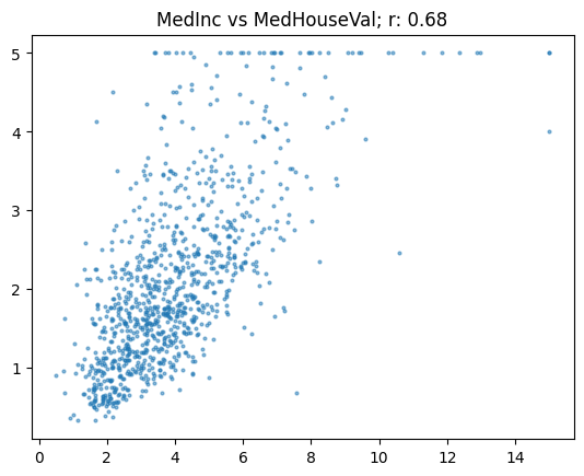

So that’s what a correlation of 0.68 looks like. It’s quite a close relationship, but there’s still a lot of variation. (Incidentally, this also shows why looking at your data is so important – we can see clearly in this plot that house prices above $500,000 seem to have been truncated to that maximum value).

Let’s take a look at another pair:

show_corr(housing, 'MedInc', 'AveRooms')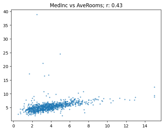

The relationship looks like it is similarly close to the previous example, but r is much lower than the income vs valuation case. Why is that? The reason is that there are a lot of outliers – values of AveRooms well outside the mean.

r is very sensitive to outliers. If there’s outliers in your data, then the relationship between them will dominate the metric. In this case, the houses with a very high number of rooms don’t tend to be that valuable, so it’s decreasing r from where it would otherwise be.

Let’s remove the outliers and try again:

subset = housing[housing.AveRooms<15]
show_corr(subset, 'MedInc', 'AveRooms')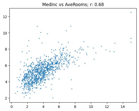

As we expected, now the correlation is very similar to our first comparison.

Here’s another relationship using AveRooms on the subset:

show_corr(subset, 'MedHouseVal', 'AveRooms')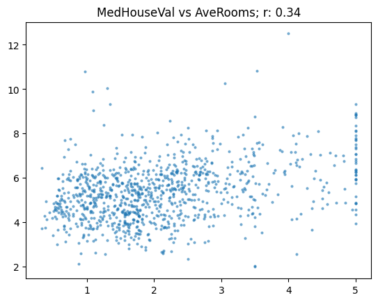

At this level, with r of 0.34, the relationship is becoming quite weak.

Let’s look at one more:

show_corr(subset, 'HouseAge', 'AveRooms')

As you see here, a correlation of -0.2 shows a very weak negative trend.

We’ve seen now examples of a variety of levels of correlation coefficient, so hopefully you’re getting a good sense of what this metric means.

Transformers expects metrics to be returned as a dict, since that way the trainer knows what label to use, so let’s create a function to do that:

def corr_d(eval_pred): return {'pearson': corr(*eval_pred)}

Training Our Model

To train a model in Transformers we’ll need this:

from transformers import TrainingArguments,Trainer

We pick a batch size that fits our GPU, and small number of epochs so we can run experiments quickly:

bs = 128
epochs = 4

The most important hyperparameter is the learning rate. fastai provides a learning rate finder to help you figure this out, but Transformers doesn’t, so you’ll just have to use trial and error. The idea is to find the largest value you can, but which doesn’t result in training failing.

lr = 8e-5

Transformers uses the TrainingArguments class to set up arguments. Don’t worry too much about the values we’re using here – they should generally work fine in most cases. It’s just the 3 parameters above that you may need to change for different models.

args = TrainingArguments('outputs', learning_rate=lr, warmup_ratio=0.1, lr_scheduler_type='cosine', fp16=True,
    evaluation_strategy="epoch", per_device_train_batch_size=bs, per_device_eval_batch_size=bs*2,
    num_train_epochs=epochs, weight_decay=0.01, report_to='none')

We can now create our model, and Trainer, which is a class which combines the data and model together (just like Learner in fastai):

model = AutoModelForSequenceClassification.from_pretrained(model_nm, num_labels=1)
trainer = Trainer(model, args, train_dataset=dds['train'], eval_dataset=dds['test'],
                  tokenizer=tokz, compute_metrics=corr_d)

Some weights of DebertaV2ForSequenceClassification were not initialized from the model checkpoint at microsoft/deberta-v3-small and are newly initialized: ['classifier.bias', 'classifier.weight', 'pooler.dense.weight', 'pooler.dense.bias']
You should probably TRAIN this model on a down-stream task to be able to use it for predictions and inference.

Let’s train our model!

trainer.train();

/usr/local/lib/python3.10/dist-packages/transformers/optimization.py:411: FutureWarning: This implementation of AdamW is deprecated and will be removed in a future version. Use the PyTorch implementation torch.optim.AdamW instead, or set `no_deprecation_warning=True` to disable this warning
  warnings.warn(
You're using a DebertaV2TokenizerFast tokenizer. Please note that with a fast tokenizer, using the `__call__` method is faster than using a method to encode the text followed by a call to the `pad` method to get a padded encoding.

[856/856 03:28, Epoch 4/4]

Epoch	Training Loss	Validation Loss	Pearson
1	No log	0.032255	0.790911
2	No log	0.023222	0.814958
3	0.040500	0.022491	0.828246
4	0.040500	0.023501	0.828109

The key thing to look at is the “Pearson” value in table above. As you see, it’s increasing, and is already above 0.8. That’s great news! We can now submit our predictions to Kaggle if we want them to be scored on the official leaderboard. Let’s get some predictions on the test set:

preds = trainer.predict(eval_ds).predictions.astype(float)
preds

array([[ 0.58],
       [ 0.69],
       [ 0.57],
       [ 0.33],
       [-0.01],
       [ 0.5 ],
       [ 0.55],
       [-0.01],
       [ 0.31],
       [ 1.15],
       [ 0.29],
       [ 0.24],
       [ 0.76],
       [ 0.91],
       [ 0.75],
       [ 0.43],
       [ 0.33],
       [-0.01],
       [ 0.66],
       [ 0.33],
       [ 0.46],
       [ 0.26],
       [ 0.18],
       [ 0.22],
       [ 0.59],
       [-0.04],
       [-0.02],
       [ 0.01],
       [-0.03],
       [ 0.59],
       [ 0.3 ],
       [-0.  ],
       [ 0.68],
       [ 0.52],
       [ 0.47],
       [ 0.23]])

Look out - some of our predictions are <0, or >1! This once again shows the value of remember to actually look at your data. Let’s fix those out-of-bounds predictions:

preds = np.clip(preds, 0, 1)

preds

array([[0.58],
       [0.69],
       [0.57],
       [0.33],
       [0.  ],
       [0.5 ],
       [0.55],
       [0.  ],
       [0.31],
       [1.  ],
       [0.29],
       [0.24],
       [0.76],
       [0.91],
       [0.75],
       [0.43],
       [0.33],
       [0.  ],
       [0.66],
       [0.33],
       [0.46],
       [0.26],
       [0.18],
       [0.22],
       [0.59],
       [0.  ],
       [0.  ],
       [0.01],
       [0.  ],
       [0.59],
       [0.3 ],
       [0.  ],
       [0.68],
       [0.52],
       [0.47],
       [0.23]])

Deeper Dive: Iterate like a grandmaster!

In this section I’ll run through the explanation and code provided in Jeremy’s notebook here.

In this notebook I’ll try to give a taste of how a competitions grandmaster might tackle the U.S. Patent Phrase to Phrase Matching competition. The focus generally should be two things:

Creating an effective validation set
Iterating rapidly to find changes which improve results on the validation set.

If you can do these two things, then you can try out lots of experiments and find what works, and what doesn’t. Without these two things, it will be nearly impossible to do well in a Kaggle competition (and, indeed, to create highly accurate models in real life!)

The more code you have, the more you have to maintain, and the more chances there are to make mistakes. So keep it simple!

from pathlib import Path
import os

iskaggle = os.environ.get('KAGGLE_KERNEL_RUN_TYPE', '')
if iskaggle:
    !pip install -Uqq fastai
else:
    import zipfile,kaggle
    path = Path('us-patent-phrase-to-phrase-matching')
    kaggle.api.competition_download_cli(str(path))
    zipfile.ZipFile(f'{path}.zip').extractall(path)

Downloading us-patent-phrase-to-phrase-matching.zip to /content

100%|██████████| 682k/682k [00:00<00:00, 1.49MB/s]

from fastai.imports import *

if iskaggle: path = Path('../input/us-patent-phrase-to-phrase-matching')
path.ls()

(#3) [Path('us-patent-phrase-to-phrase-matching/sample_submission.csv'),Path('us-patent-phrase-to-phrase-matching/test.csv'),Path('us-patent-phrase-to-phrase-matching/train.csv')]

Let’s look at the training set:

df = pd.read_csv(path/'train.csv')
df

	id	anchor	target	context	score
0	37d61fd2272659b1	abatement	abatement of pollution	A47	0.50
1	7b9652b17b68b7a4	abatement	act of abating	A47	0.75
2	36d72442aefd8232	abatement	active catalyst	A47	0.25
3	5296b0c19e1ce60e	abatement	eliminating process	A47	0.50
4	54c1e3b9184cb5b6	abatement	forest region	A47	0.00
...	...	...	...	...	...
36468	8e1386cbefd7f245	wood article	wooden article	B44	1.00
36469	42d9e032d1cd3242	wood article	wooden box	B44	0.50
36470	208654ccb9e14fa3	wood article	wooden handle	B44	0.50
36471	756ec035e694722b	wood article	wooden material	B44	0.75
36472	8d135da0b55b8c88	wood article	wooden substrate	B44	0.50

36473 rows × 5 columns

And the test set:

eval_df = pd.read_csv(path/'test.csv')
len(eval_df)

eval_df.head()

	id	anchor	target	context
0	4112d61851461f60	opc drum	inorganic photoconductor drum	G02
1	09e418c93a776564	adjust gas flow	altering gas flow	F23
2	36baf228038e314b	lower trunnion	lower locating	B60
3	1f37ead645e7f0c8	cap component	upper portion	D06
4	71a5b6ad068d531f	neural stimulation	artificial neural network	H04

df.target.value_counts()

composition                    24
data                           22
metal                          22
motor                          22
assembly                       21
                               ..
switching switch over valve     1
switching switch off valve      1
switching over valve            1
switching off valve             1
wooden substrate                1
Name: target, Length: 29340, dtype: int64

We see that there’s nearly as many unique targets as items in the training set, so they’re nearly but not quite unique. Most importantly, we can see that these generally contain very few words (1-4 words in the above sample).

df.anchor.value_counts()

component composite coating              152
sheet supply roller                      150
source voltage                           140
perfluoroalkyl group                     136
el display                               135
                                        ... 
plug nozzle                                2
shannon                                    2
dry coating composition1                   2
peripheral nervous system stimulation      1
conduct conducting material                1
Name: anchor, Length: 733, dtype: int64

We can see here that there’s far fewer unique values (just 733) and that again they’re very short (2-4 words in this sample).

df.context.value_counts()

H01    2186
H04    2177
G01    1812
A61    1477
F16    1091
       ... 
B03      47
F17      33
B31      24
A62      23
F26      18
Name: context, Length: 106, dtype: int64

The first character is the section the patent was filed under – let’s create a column for that and look at the distribution:

df['section'] = df.context.str[0]
df.section.value_counts()

B    8019
H    6195
G    6013
C    5288
A    4094
F    4054
E    1531
D    1279
Name: section, dtype: int64

Finally, we’ll take a look at a histogram of the scores:

df.score.hist();

There’s a small number that are scored 1.0 - here’s a sample:

df[df.score==1]

	id	anchor	target	context	score	section
28	473137168ebf7484	abatement	abating	F24	1.0	F
158	621b048d70aa8867	absorbent properties	absorbent characteristics	D01	1.0	D
161	bc20a1c961cb073a	absorbent properties	absorption properties	D01	1.0	D
311	e955700dffd68624	acid absorption	absorption of acid	B08	1.0	B
315	3a09aba546aac675	acid absorption	acid absorption	B08	1.0	B
...	...	...	...	...	...	...
36398	913141526432f1d6	wiring trough	wiring troughs	F16	1.0	F
36435	ee0746f2a8ecef97	wood article	wood articles	B05	1.0	B
36440	ecaf479135cf0dfd	wood article	wooden article	B05	1.0	B
36464	8ceaa2b5c2d56250	wood article	wood article	B44	1.0	B
36468	8e1386cbefd7f245	wood article	wooden article	B44	1.0	B

1154 rows × 6 columns

We can see from this that these are just minor rewordings of the same concept, and isn’t likely to be specific to context. Any pretrained model should be pretty good at finding these already.

Training

! pip install transformers[sentencepiece] datasets accelerate

from torch.utils.data import DataLoader
import warnings,transformers,logging,torch
from transformers import TrainingArguments,Trainer
from transformers import AutoModelForSequenceClassification,AutoTokenizer

if iskaggle:
    !pip install -q datasets
import datasets
from datasets import load_dataset, Dataset, DatasetDict

# quiet huggingface warnings
warnings.simplefilter('ignore')
logging.disable(logging.WARNING)

# specify which model we are going to be using
model_nm = 'microsoft/deberta-v3-small'

We can now create a tokenizer for this model. Note that pretrained models assume that text is tokenized in a particular way. In order to ensure that your tokenizer matches your model, use the AutoTokenizer, passing in your model name.

tokz = AutoTokenizer.from_pretrained(model_nm)

We’ll need to combine the context, anchor, and target together somehow. There’s not much research as to the best way to do this, so we may need to iterate a bit. To start with, we’ll just combine them all into a single string. The model will need to know where each section starts, so we can use the special separator token to tell it:

sep = tokz.sep_token
sep

'[SEP]'

df['inputs'] = df.context + sep + df.anchor + sep + df.target

Generally we’ll get best performance if we convert pandas DataFrames into HuggingFace Datasets, so we’ll convert them over, and also rename the score column to what Transformers expects for the dependent variable, which is label:

ds = Dataset.from_pandas(df).rename_column('score', 'label')
eval_ds = Dataset.from_pandas(eval_df)

To tokenize the data, we’ll create a function (since that’s what Dataset.map will need):

def tok_func(x): return tokz(x["inputs"])

tok_func(ds[0])

{'input_ids': [1, 336, 5753, 2, 47284, 2, 47284, 265, 6435, 2], 'token_type_ids': [0, 0, 0, 0, 0, 0, 0, 0, 0, 0], 'attention_mask': [1, 1, 1, 1, 1, 1, 1, 1, 1, 1]}

The only bit we care about at the moment is input_ids. We can see in the tokens that it starts with a special token 1 (which represents the start of text), and then has our three fields separated by the separator token 2. We can check the indices of the special token IDs like so:

tokz.all_special_tokens

['[CLS]', '[SEP]', '[UNK]', '[PAD]', '[MASK]']

We can now tokenize the input. We’ll use batching to speed it up, and remove the columns we no longer need:

inps = "anchor","target","context"
tok_ds = ds.map(tok_func, batched=True, remove_columns=inps+('inputs','id','section'))

Looking at the first item of the dataset we should see the same information as when we checked tok_func above:

tok_ds[0]

{'label': 0.5,
 'input_ids': [1, 336, 5753, 2, 47284, 2, 47284, 265, 6435, 2],
 'token_type_ids': [0, 0, 0, 0, 0, 0, 0, 0, 0, 0],
 'attention_mask': [1, 1, 1, 1, 1, 1, 1, 1, 1, 1]}

Creating a validation set

According to this post, the private test anchors do not overlap with the training set. So let’s do the same thing for our validation set.

First, create a randomly shuffled list of anchors:

anchors = df.anchor.unique()
np.random.seed(42)
np.random.shuffle(anchors)
anchors[:5]

array(['time digital signal', 'antiatherosclerotic', 'filled interior',
       'dispersed powder', 'locking formation'], dtype=object)

Now we can pick some proportion (e.g 25%) of these anchors to go in the validation set:

val_prop = 0.25
val_sz = int(len(anchors)*val_prop)
val_anchors = anchors[:val_sz]

Now we can get a list of which rows match val_anchors, and get their indices:

# is_val is a boolean array
is_val = np.isin(df.anchor, val_anchors)
idxs = np.arange(len(df))
val_idxs = idxs[ is_val]
trn_idxs = idxs[~is_val]
len(val_idxs),len(trn_idxs)

(9116, 27357)

Our training and validation Datasets can now be selected, and put into a DatasetDict ready for training:

dds = DatasetDict({"train":tok_ds.select(trn_idxs),
             "test": tok_ds.select(val_idxs)})

BTW, a lot of people do more complex stuff for creating their validation set, but with a dataset this large there’s not much point. As you can see, the mean scores in the two groups are very similar despite just doing a random shuffle:

df.iloc[trn_idxs].score.mean(),df.iloc[val_idxs].score.mean()

(0.3623021530138539, 0.3613426941641071)

Initial model

Let’s now train our model! We’ll need to specify a metric, which is the correlation coefficient provided by numpy (we need to return a dictionary since that’s how Transformers knows what label to use):

def corr(eval_pred): return {'pearson': np.corrcoef(*eval_pred)[0][1]}

We pick a learning rate and batch size that fits our GPU, and pick a reasonable weight decay and small number of epochs:

lr,bs = 8e-5,128
wd,epochs = 0.01,4

Transformers uses the TrainingArguments class to set up arguments. We’ll use a cosine scheduler with warmup, since at fast.ai we’ve found that’s pretty reliable. We’ll use fp16 since it’s much faster on modern GPUs, and saves some memory. We evaluate using double-sized batches, since no gradients are stored so we can do twice as many rows at a time.

def get_trainer(dds):
    args = TrainingArguments('outputs', learning_rate=lr, warmup_ratio=0.1, lr_scheduler_type='cosine', fp16=True,
        evaluation_strategy="epoch", per_device_train_batch_size=bs, per_device_eval_batch_size=bs*2,
        num_train_epochs=epochs, weight_decay=wd, report_to='none')
    model = AutoModelForSequenceClassification.from_pretrained(model_nm, num_labels=1)
    return Trainer(model, args, train_dataset=dds['train'], eval_dataset=dds['test'],
                   tokenizer=tokz, compute_metrics=corr)

args = TrainingArguments('outputs', learning_rate=lr, warmup_ratio=0.1, lr_scheduler_type='cosine', fp16=True,
    evaluation_strategy="epoch", per_device_train_batch_size=bs, per_device_eval_batch_size=bs*2,
    num_train_epochs=epochs, weight_decay=wd, report_to='none')

We can now create our model, and Trainer, which is a class which combines the data and model together (just like Learner in fastai):

model = AutoModelForSequenceClassification.from_pretrained(model_nm, num_labels=1)
trainer = Trainer(model, args, train_dataset=dds['train'], eval_dataset=dds['test'],
               tokenizer=tokz, compute_metrics=corr)

trainer.train();

[856/856 03:02, Epoch 4/4]

Epoch	Training Loss	Validation Loss	Pearson
1	No log	0.027171	0.794542
2	No log	0.026872	0.811033
3	0.035300	0.024633	0.816882
4	0.035300	0.024581	0.817413

Improving the model

We now want to start iterating to improve this. To do that, we need to know whether the model gives stable results. I tried training it 3 times from scratch, and got a range of outcomes from 0.808-0.810. This is stable enough to make a start - if we’re not finding improvements that are visible within this range, then they’re not very significant! Later on, if and when we feel confident that we’ve got the basics right, we can use cross validation and more epochs of training.

Iteration speed is critical, so we need to quickly be able to try different data processing and trainer parameters. So let’s create a function to quickly apply tokenization and create our DatasetDict:

def get_dds(df):
    ds = Dataset.from_pandas(df).rename_column('score', 'label')
    tok_ds = ds.map(tok_func, batched=True, remove_columns=inps+('inputs','id','section'))
    return DatasetDict({"train":tok_ds.select(trn_idxs), "test": tok_ds.select(val_idxs)})

def get_model(): return AutoModelForSequenceClassification.from_pretrained(model_nm, num_labels=1)

def get_trainer(dds, model=None):
    if model is None: model = get_model()
    args = TrainingArguments('outputs', learning_rate=lr, warmup_ratio=0.1, lr_scheduler_type='cosine', fp16=True,
        evaluation_strategy="epoch", per_device_train_batch_size=bs, per_device_eval_batch_size=bs*2,
        num_train_epochs=epochs, weight_decay=wd, report_to='none')
    return Trainer(model, args, train_dataset=dds['train'], eval_dataset=dds['test'],
                   tokenizer=tokz, compute_metrics=corr)

Perhaps using the special separator character isn’t a good idea, and we should use something we create instead. Let’s see if that makes things better. First we’ll change the separator and create the DatasetDict:

sep = " [s] "
df['inputs'] = df.context + sep + df.anchor + sep + df.target
dds = get_dds(df)

get_trainer(dds).train()

[856/856 03:27, Epoch 4/4]

Epoch	Training Loss	Validation Loss	Pearson
1	No log	0.027216	0.799765
2	No log	0.025568	0.814325
3	0.031000	0.023474	0.817759
4	0.031000	0.024206	0.817377

TrainOutput(global_step=856, training_loss=0.023552694610346144, metrics={'train_runtime': 207.9058, 'train_samples_per_second': 526.335, 'train_steps_per_second': 4.117, 'total_flos': 582121520370810.0, 'train_loss': 0.023552694610346144, 'epoch': 4.0})

That’s looking quite a bit better, so we’ll keep that change.

(Vishal note: I trained it a few times but couldn’t get the pearson coefficient past 0.8174)

Often changing to lowercase is helpful. Let’s see if that helps too:

df['inputs'] = df.inputs.str.lower()
dds = get_dds(df)
get_trainer(dds).train()

[755/856 02:53 < 00:23, 4.33 it/s, Epoch 3.52/4]

Epoch	Training Loss	Validation Loss	Pearson
1	No log	0.025207	0.798847
2	No log	0.024926	0.813183
3	0.031800	0.023556	0.815640

[856/856 03:17, Epoch 4/4]

Epoch	Training Loss	Validation Loss	Pearson
1	No log	0.025207	0.798847
2	No log	0.024926	0.813183
3	0.031800	0.023556	0.815640
4	0.031800	0.024359	0.815295

TrainOutput(global_step=856, training_loss=0.024133934595874536, metrics={'train_runtime': 197.3858, 'train_samples_per_second': 554.386, 'train_steps_per_second': 4.337, 'total_flos': 582121520370810.0, 'train_loss': 0.024133934595874536, 'epoch': 4.0})

Special tokens

What if we made the patent section a special token? Then potentially the model might learn to recognize that different sections need to be handled in different ways. To do that, we’ll use, e.g. [A] for section A. We’ll then add those as special tokens:

df['sectok'] = '[' + df.section + ']'
sectoks = list(df.sectok.unique())
tokz.add_special_tokens({'additional_special_tokens': sectoks})

df['inputs'] = df.sectok + sep + df.context + sep + df.anchor.str.lower() + sep + df.target
dds = get_dds(df)

Since we’ve added more tokens, we need to resize the embedding matrix in the model:

model = get_model()
model.resize_token_embeddings(len(tokz))

Embedding(128009, 768)

trainer = get_trainer(dds, model=model)
trainer.train()

[856/856 03:41, Epoch 4/4]

Epoch	Training Loss	Validation Loss	Pearson
1	No log	0.025942	0.810038
2	No log	0.025694	0.814332
3	0.010500	0.023547	0.816508
4	0.010500	0.024562	0.817200

TrainOutput(global_step=856, training_loss=0.009868621826171875, metrics={'train_runtime': 221.7169, 'train_samples_per_second': 493.548, 'train_steps_per_second': 3.861, 'total_flos': 695370741753690.0, 'train_loss': 0.009868621826171875, 'epoch': 4.0})

Before submitting a model, retrain it on the full dataset, rather than just the 75% training subset we’ve used here. Create a function like the ones above to make that easy for you!

Video Notes

In this section, I’ll take notes while watching this lesson’s video.

Introduction
- In the book, we do NLP using Recurrent Neural Networks (RNNs).
- In the video, we’re going to be fine-tuning a pretrained NLP model using a library called HuggingFace Transformers.
- It’s useful to have experience in using more than one library. See the same concepts applied in different ways. Great for understanding the concepts.
- HuggingFace libraries are SOTA in NLP.
- Transformers library in process of being integrated into fastai library.
- HuggingFace Transformers doesn’t have the same layered API as fastai.
Fine-Tuning a Pretrained Model
- In the quadratic/sliders example, a pretrained model is like someone telling you that they are confident what parameter a should be, are somewhat confident what b should be, and have no idea what c should be. Then, we would train c until it firts our model, adjust b and keep a as is. That’s what it’s like fine-tuning a pretrained model.
- A pretrained model is a bunch of parameters have already been fit, where for some of them we’re pretty confident of what they should be, and for some of them we really have no idea at all.
- Fine-tuning is the process of taking those ones where we have no idea at all what they should be and trying to get them right, and then moving the other ones a little bit.
ULMFiT
- The idea of fine-tuning a pretrained NLP model was pioneered by ULMFiT which was first introduced in a fastai course, later turned into an academic paper by Jeremy and Sebastian Ruder which inspired a huge change in NLP capabilities around the world.
- Step 1
  - Build a language model using all of Wikipedia that tried to predict the next word of a Wikipedia article. Filling in these kinds of things requires understanding a lot about how language is structured and about the world. Getting good at fitting a language model requires a neural net getting good at a lot of things. It needs to understand language at a reasonably good level, what is true, what is not true, different ways in which things are expressed and so on. Started with random weights. At the end was a model that could predict more than 30% of the time correctly what the next word in a Wikipedia article would be.
- Step 2
  - Create a second language model, that predicts the next word of a sentence. Took the pretrained model and ran a few more epochs using IMDb movie reviews. So it got very good at predicting the next work of an IMDb movie review.
- Step 3
  - Took those weights and fine-tuned them for the task of predicting whether or not a movie review was positive or negative sentiment.
The first two models don’t require labels. The labels was what’s the next word of the sentence.
ULMFiT built with RNNs.
Transformers developed at the same time of ULMFiT’s release.
Transformers can take advantage of modern accelerators like Google’s TPUs.
Transformers don’t allow you to predict the next word of a sentence, it’s just not how they are structured. Instead they deleted at random a few words and asked the model to predict what words were deleted. The basic concept similar to ULMFiT ,replaced RNN with Transformer. Replaced language model with masked language model.
How do you go from a model that’s trained to predict the next word to a model that does classification?
- The first layer of ImageNet classification model finds basic features like diagonal edges, gradients, etc. Layer two combined those (ReLUs added together, activations from sets of ReLUs matrix multipled, etc.)
- Layer 5 had bird and lizard eyeball detectors, dog face detectors, flowers detectors, etc.
- Later layers do things much more specific to the training task.
- Pretty unlikely that you need to change the early layers.
- The layer that says “what is this” is deleted in fine-tuning (the layer that has one output per category). The model is then spitting out a few hundred activations. We stick a new random matrix on top of that and train it, so it can predict what you’re trying to predict. Then we gradually train the rest of the layers.
Getting started with NLP for absolute beginners
- US Patent Phrase to Phrase Matching Competition.
- Classification is probably the most widely use case for NLP.
- Document = an input to an NLP model that contains text.
- Classifying a document is a rich thing to do: sentiment analysis, author identifiation, legal discovery, organizing documents by topic, triaging inbound emails.
- The Kaggle competition on US Patents does not immediately look like a classification problem.
- Columns: Anchor, target, context, score
- Goal: come up with a model that automatically determines which anchor and target pairs are talking about the same thing. score = 1.0 means the anchor and target mean the same thing, 0.0 means they are not.
- Whether the anchor and target are determined to be similar or not depends on the context.
- Represent the problem as <constant string><anchor><seperator><constant string><target> and choose category 0.0, 0.25, 0.50, 0.75 or 1.00.
- Kaggle data is already on Kaggle.
- Always look through the competition’s Data page and read through it before jumping into the data.
- Use DataFrame.describe(include='object') to see stats about the fields (count, unique, top, frequency of top).
- This dataset contains very small documents (3-4 words) that are not very unique. There’s not a lot of unique data to work with.
- Create a single string of anchor, target, and context with separators and store as the input column.
- Neural networks work with numbers: We’re going to take the numbers, multiply by matrices, replace negatives with zeros, add them up, and do this a few times.
  - Tokenization: Split each document into tokens (words).
  - The list of unique words is called the vocabulary.
  - Numericalization: Each word in the vocabulrary gets a number. The bigger the vocab, the more memory gets used, the more data we need to train. We don’t want a large vocabulary.
  - Tokenize into sub-words (pieces of words).
- We can turn a pandas DataFrame into a Huggingface dataset’s Dataset using Dataset.from_pandas.
- Whatever pretrained model you used comes with a tokenizer. Before you start tokenizing, you have to decide on which model to use.
- Hugginface Model Hub has pretrained models trained on specific corpuses.
- There are some generally good models, deberta-v3 is one of those.
- NLP has been practically effective for general users for only a year or two, a lot of this stuff we’re figuring out as a community.
- Always start with a small model, it’s faster to train, we’re going to be able to do more iterations.
- AutoTokenizer.from_pretrained(<model name>) will download the vocab and details about how this particular model tokenized the dataset.
- _ represents the start of a word.
- def tok_func(x): return tokx(x['input']) takes a document x, and tokenizes it’s input.
- Dataset.map will parallelize the process of calling the function on each value. batched=True will do a bunch at a time. Tokenizer library is an optimized Rust library.
- input_ids will contain numbers in the position of each of the tokens.
- How do you choose the keywords and the order of the fields when creating input?
  - It’s arbitrary, try a few things. We just want something it can learn from that separates one field from another.
- If one of the fields was long (1000 characters) is there any special handling required there?
  - Long documents in ULMFiT require no special consideration. ULMFiT is the best approach for large documents. It will split large documents into pieces.
  - Large documents are challening for Transformers. It does the whole document at once.
  - Documents over 2000 words: look at ULMFiT.
  - Under 2000 words: Transformers should be fine unless you have a laptop GPU with not much memory.
- HuggingFace transformers expect that your target is a column called labels.
- test.csv doesn’t have a score field.
- Perhaps the most important idea in machine learning is having separate training, validation and test datasets.
- Test and validation sets are all about identifying and controlling for overfitting.
- Underfit: not enough complexity in the model fit to match the data that’s there. It’s systematically biased.
- Common misunderstanding is that simpler models are more reliable in some way, but models that are too simple will be systematically incorrect.
- Overfit: it’s done a good job of fitting our data points, but if we sample some more data points from our distribution the model won’t be close to them.
- Underfitting is easy to recognize (we can look at training data and see that it’s not very close).
- Overfitting is harder to recognize because the training data is very close.
- How do we tell if we have a good fit that’s not overfitting? We measure how good our model is by looking ONLY at the points we set aside as the validation set.
- fast.ai won’t let you train a model without a validation set and shows metrics only on the validation set.
- Creating a good validation set is not generally as simple as just randomly pulling some of your data out of the data that you train your model on.
- Kaggle is a great place to learn how to create a good validation set.
- A test set is another validation set that you don’t use for metrics. Helps you see if you overfit using the validation set.
- Kaggle has two test sets: leaderboard feedback during competition and second test set that is private until after competition is finished.
- Don’t accidentally find a model that is good by coincidence. Only if you have a test set that you hold out will you know if you’ve done this.
- If your model is terrible on the test set—go back to square one.
- You don’t want functions with gradient of 0 of inf (like accuracy) you want something smooth.
- One metric is not enough to capture all of the real world dynamics involved in a model’s use.
- Goodhart’s law: when a measure becomes a target, it’s ceases to be a good measure.
- AI is really good at optimizing metrics so you have to be careful what metrics you choose for models that are used in real life (impacting people’s lives).
- Pearson correlation coefficient is the most widely used measure of how similar two variables are
  - -1.0 to +1.0.
  - Abbreviated as r.
- How do I plot datasets with far too many points? The answer is: get less points (sample).
- np.corrcoef gives a diagonally symmetric matrix of r values.
- Visualizing your data is important so you can see things like how data is truncated.
- alpha=0.5 for scatter plots creates darker areas where there’s lots of dots.
- r relies on the square of the difference, big outliers increase that by a lot.
- r is very sensitive to outliers.
- If you’re trying to win a Kaggle competition that uses r and even a couple of your rows are really wrong, it will be a disaster.
- You almost can’t see the relationship for $r=0.34$
- Transformers expects metric to be returned as a dict.
- tok_ds.train_test_split() returns a DatasetDict({train: Dataset, test: Dataset}).
- Transformers calls it validation set test, on which is calculates metrics.
- The fastai equivalent of Learner is the HuggingFace Transformer’s Trainer.
- The larger the batch size, the more you can do in parallel and the faster it’ll be, but if it’s too large you’ll get an out-of-memory error on the GPU.
- If you’re using a framework that doesn’t have a learning rate finder like fastai, you can just start with a really low learning rate and then keep doubling it until it falls apart.
- TrainingArguments is a class that takes all of the configuration (like learning rate, warmup ratio, scheduler type, weight decay, etc.).
- You always want fp16=True as it will be faster.
- AutoModelForSequenceClassification will create an model for classification, .from_pretrained will use a pretrained model which has a num_labels param which is the number of output columns we have, which in this case is 1 (the score).
- Trainer takes the model, the training and validation data, TrainingArguments(), tokenizer and metrics).
- Trainer.train() will train the model.
- HuggingFace is very verbose, the warnings which you can ignore.
- The only reason we get a high r value after 4 epochs is because we used a pretrained model.
- The pretrained model already knows a lot about language and has a good sense of whether two phrases have the same meaning or not.
- How do you decide when it’s okay to remove outliers?
  - Outliers should never just be removed for modelling.
  - Instead we would observe that clearly from looking at this dataset, these two groups can’t be treated the same way (low income/high # of rooms vs. high income/high # of rooms). Split them into two separate analyses.
  - Outlier exists in a statistical sense, it doesn’t exist in a real sense (i.e. things that we should ignore or throw away). Some of the most useful insights in data projects are digging into outliers and understanding what are they? and where did they come from? It’s in those edge cases where you discover really important things like when processes go wrong, labelling problems. Never delete outliers. Investigate them, have a strategy about what you’re going to do with them.
- Training with HuggingFace’s Transformer is similar to the things we’ve seen before with fastai.
- trainer.predict(eval_ds).predictions.astype(float) to get predictions from Trainer object.
- Always look at your outputs. So you can see things like having negative predictions or predictions over 1, which are outside the range of the patent phrase matching score. For now, we can at least round these off up to 0 and down to 1, respectively, better ways to do this but this is better than nothing.
- Kaggle expects submissions to generally be in a CSV file.
- NLP is probably where the biggest opportunities are for big wins in research and commercialization.
It’s worth thinking about both use and misuse of modern NLP.
You can create bots to generate context appropriate conversation and scale it up to 99% of Twitter and nobody would know. This is worrying because a lot of how people see the world is coming out of social media conversation, which at this point are contrallable. It would not be that hard to create something that’s optimized towards moving a point of view amongst a billion people in a very subtle way, very gradually over a long period of time by multiple bots each pretending to argue with each other and one of them getting the upper hand and so forth.
What GPT is used for we may not know for decades, if ever.
2017: millions of submissions to the FTC about Net Neutrality very heavily biased against it. An analysis showed that something like 99% of them were auto-generated. We don’t know for sure but this seems successful because repealing Net Neutrality went through, the comments were factored into this decision.
You can always create a generative model that beats bot classifiers designed to classify its content as auto-generated. Similar problem with spam prevention.
If you pass num_labels=1 to AutoModelForSequenceClassification it treats it as a regression problem.

Book Notes

In this section, I’ll take notes and run code examples from Chapter 10: NLP Deep Dive: RNNs in the textbook.

In general, in NLP the pretrained model is trained on a different task.
language model: a model that has been trained to guess the next word in a text (having read the ones before).
self-supervised learning: Training a model using labels that are embedded in the independent variable, rather than requiring external labels.
To properly guess the next word in a sentence, the model will have to develop an understanding of the natural language.
Self-supervised learning is not usually used for the model that is trained directly, but instead is used for pretraining a model used for transfer learning.
Self-supervised learning and computer vision
Even if our language model knows the basics of the language we are using in the task (e.g., our pretrained model is in English), it helps to get used to the style of the corpus we are targeting.
You get even better results if you fine-tune the sequence-based language model prior to fine-tuning the classification model.
The IMDb dataset contains 100k movie reviews (50k unlabeled, 25k labeled training set reviews, 25k labeled validation set reviews). We can use all of these reviews to fine-tune the pretrained language model, which was trained only on Wikipedia articles, this will result in a language model that is particularly good at predicting the next word of a movie review. This is known as Universal Language Model Fine-tuning (ULMFiT).
The extra stage of fine-tuning the language model, prior to transfer learning to classification task, resulted in significantly better predictions.

Text Preprocessing

Using categorical variables as independent variables for a neural network:
- Make a list of all possible levels of that categorical variable (the vocab).
- Replace each level with its index in the vocab.
- Create an embedding matrix for this containing a row for each level (i.e., for each item of the vocab).
- Use this embedding matrix as the first layer of a neural network. (A dedicated embedding matrix can take as inputs the raw vocab indexes created in step 2; this is equivalent to, but faster and more efficient than, a matrix that takes as input one-hot-encoded vectors representing the indexes).
We can do nearly the same thing with text:
- First we concatenate all of the documents in our dataset into one big long string and split it into words (or tokens), giving us a very long list of words.
- Our independent variable will be the sequence of words starting with the first word in our very long list and ending with the second to last, and our dependent variable will be the sequence of words starting with the second word and ending with the last word.
- Our vocab will consist of a mix of common words that are already in the vocabulary of our pretrained model and new words specific to our corpus.
- Our embedding matrix will be built accordingly: for words that are in the vocabulary of our pretrained model, we will take the corresponding row in the embedding matrix of the pretrained model; but for new words, we won’t have anything, so we will just initialize the corresponding row with a random vector.
Steps for creating a language model:
- Tokenization: convert the text into a list of words (or characters, or substrings, depending on the granularity of your model)
- Numericalization: List all of the unique words that appear (vocab) and convert each word into a number by looking up its index in the vocab.
- Language model data loader creation: fastai’s LMDataLoader automatically handles creating a dependent variable that is offset from the independent variable by one token, and handles important details liks shuffling the training data so that the dependent and independent variables maintain their structure as required.
- Language model creation: we need a model that handles input lists that could be arbitrarily big or small. We use a Recurrent Neural Network (RNN).

Tokenization

There is no one approach to tokenization. There are three main approaches:

Word-based: Split a sentence on spaces and separate parts of meaning even when there are no spaces (“don’t” -> “do n’t”). Punctuation marks are generally split into separate tokens.
Subword based: Split words into smaller parts, based on the most commonly occurring substrings (“occasion” -> “o c ca sion”).
Character-based: Split a sentence into its individual characters.

Word Tokenization with fastai

Rather than providing its own tokenizers, fastai provides a consistent interface to a range of tokenizers in external libraries.

Let’s try it out with the IMDb dataset:

from fastai.text.all import *
path = untar_data(URLs.IMDB)

100.00% [144441344/144440600 00:02<00:00]

path.ls()

(#7) [Path('/root/.fastai/data/imdb/unsup'),Path('/root/.fastai/data/imdb/tmp_lm'),Path('/root/.fastai/data/imdb/imdb.vocab'),Path('/root/.fastai/data/imdb/test'),Path('/root/.fastai/data/imdb/tmp_clas'),Path('/root/.fastai/data/imdb/train'),Path('/root/.fastai/data/imdb/README')]

get_text_files gets all the text files in a path

files = get_text_files(path, folders = ['train', 'test', 'unsup'])

files[:10]

(#10) [Path('/root/.fastai/data/imdb/unsup/42765_0.txt'),Path('/root/.fastai/data/imdb/unsup/19120_0.txt'),Path('/root/.fastai/data/imdb/unsup/8649_0.txt'),Path('/root/.fastai/data/imdb/unsup/32022_0.txt'),Path('/root/.fastai/data/imdb/unsup/30143_0.txt'),Path('/root/.fastai/data/imdb/unsup/14876_0.txt'),Path('/root/.fastai/data/imdb/unsup/28162_0.txt'),Path('/root/.fastai/data/imdb/unsup/32133_0.txt'),Path('/root/.fastai/data/imdb/unsup/21844_0.txt'),Path('/root/.fastai/data/imdb/unsup/830_0.txt')]

Here’s a review that we will tokenize:

txt = files[0].open().read(); txt[:75]

"Despite some humorous banter and a decent supporting cast, I can't really r"

WordTokenizer will always point to fastai’s current default word tokenizer.

fastai’s coll_repr(collection, n) displays the first n items of collection, along with the full size.

tokz = WordTokenizer()
toks = first(tokz([txt]))
print(coll_repr(toks, 30))

(#243) ['Despite','some','humorous','banter','and','a','decent','supporting','cast',',','I','ca',"n't",'really','recommend','this','movie','.','The','leads','are',"n't",'very','likable','and','I','did',"n't",'particularly','care'...]

Tokenization is a surprisingly subtle task. “.” is separated when it terminates a sentence but not in an acronym or number:

first(tokz(['The U.S. dollar $1 is $1.00.']))

(#9) ['The','U.S.','dollar','$','1','is','$','1.00','.']

fastai adds some functionality to the tokenization process with the Tokenizer class:

tkn = Tokenizer(tokz)
print(coll_repr(tkn(txt), 31))

(#264) ['xxbos','xxmaj','despite','some','humorous','banter','and','a','decent','supporting','cast',',','i','ca',"n't",'really','recommend','this','movie','.','xxmaj','the','leads','are',"n't",'very','likable','and','i','did',"n't"...]

Tokens that start with xx are special tokens.

xxbos is a special token that indicates the start of a new text (“BOS” is a standard NLP acronym that means “beginning of stream”). By recognizing this start token, the model will be able to learn it needs to “forget” what was said previously and focus on upcoming words. These special tokens don’t come from the external tokenizer. fastai adds them by default by applying a number of rules when processing text. These rules are designed to make it easier for a model to recognize the important parts of a sentence. We are translating the original English language sequence into a simplified tokenized language that is designed to be easy for a model to learn.

For example, the rules will replace a sequence of four exclamation points with a single exclamation point follow by a special repeated character token and then the number four.

tkn('!!!!')

(#4) ['xxbos','xxrep','4','!']

In this way, the model’s embedding matrix can encode information about general concepts such as repeated punctuation rather than requiring a separate token for every number of repititions of every punctuation mark. A capitalized word will be replaced with a special capitalization token, followed by the lowercase version of the word so the embedding matrix needs only the lowercase version of the words saving compute and memory resources but can still learn the concept of capitalization.

Here are some of the main special tokens:

xxbos: Indicates the beginning of a text (in this case, a review).

xxmaj: Indicates the next word begins with a capital.

xxunk: Indicates the next word is unknown.

defaults.text_proc_rules

[<function fastai.text.core.fix_html(x)>,
 <function fastai.text.core.replace_rep(t)>,
 <function fastai.text.core.replace_wrep(t)>,
 <function fastai.text.core.spec_add_spaces(t)>,
 <function fastai.text.core.rm_useless_spaces(t)>,
 <function fastai.text.core.replace_all_caps(t)>,
 <function fastai.text.core.replace_maj(t)>,
 <function fastai.text.core.lowercase(t, add_bos=True, add_eos=False)>]

fix_html: replaces special HTML characters with a readable version.

replace_rep: Replaces any character repeated three times or more with a special token for repetition (xxrep), the number of times it’s repeated, then the character.

replace_wrep: Replaces any word repeated three times or more with a special token for word repetition (xxwrep), the number of times it’s repeated, then the character.

spec_add_spaces: adds spaces around / and #.

rm_useless_spaces: Removes all repetitions of the space character.

replace_all_caps: Lowercases a word written in all caps and adds a special token for all caps (xxcap) in front of it.

replace_maj: Lowercases a capitalized word and adds a special token for capitalized (xxmaj) in front of it.

lowercase: Lowercases all text and adds a special token at the beginning (xxbos) and/or the end (xxeos).

coll_repr(tkn("&copy;    Fast.ai www.fast.ai/INDEX"), 31)

"(#11) ['xxbos','©','xxmaj','fast.ai','xxrep','3','w','.fast.ai','/','xxup','index']"

Subword Tokenization

Word tokenization relies on an assumption that spaces provide a useful separation of components of meaning in a sentence. However this assumption is not always appropriate. Languages like Chinese and Japanese don’t use spaces. Turkish and Hungarian can add many subwords together without spaces.

Two steps of subword tokenization:

Analyze a corpus of documents to find the most commonly occuring groups of letters. These becomes the vocab.
Tokenize the corpus string using this vocab of subword units.

txts = L(o.open().read() for o in files[:2000])

! pip install sentencepiece
def subword(sz):
  sp = SubwordTokenizer(vocab_sz=sz)
  sp.setup(txts)
  return ' '.join(first(sp([txt]))[:40])

setup reads the documents and finds the common sequences of characters to create the vocab.

subword(1000)

"▁De s p ite ▁some ▁humor ous ▁b ant er ▁and ▁a ▁de cent ▁support ing ▁cast , ▁I ▁can ' t ▁really ▁recommend ▁this ▁movie . ▁The ▁lead s ▁are n ' t ▁very ▁li k able ▁and ▁I"

When using fastai’s subword tokenizer, _ represents a space character in the original text.

If we use a smaller vocab, each token will represent fewer characters and it will take more tokens to represent a sentence.

subword(200)

'▁ D es p it e ▁ s o m e ▁h u m or o us ▁b an ter ▁and ▁a ▁ d e c ent ▁ s u p p or t ing ▁ c a s t'

If we use a larger vocab, most common English words will end up in the vocab themselves, and we will not need as many to represent a sentence:

subword(10000)

"▁Des pite ▁some ▁humorous ▁ban ter ▁and ▁a ▁decent ▁support ing ▁cast , ▁I ▁can ' t ▁really ▁recommend ▁this ▁movie . ▁The ▁leads ▁are n ' t ▁very ▁likable ▁and ▁I ▁didn ' t ▁particular ly ▁care ▁if ▁they"

A larger vocab means fewer tokens per sentence, which means faster training, less memory and less state for the model to remember; but on the downside, it means larger embedding matricces, which require more data to learn.

Subword tokenization provides a way to easily scale between character tokenization (using a small subword vocab) and word tokenization (using a large subword vocab) and handles every human language. It can even handle genomic sequences or MIDI music notation. It’s likely to become (or has already) the most common tokenization approach.

Numericalization with fast.ai

Numericalization is the process of mapping tokens to integers.

Make a list of all possible levels of the categorical variable (the vocab).
Replace each level with its index in the vocab.

toks = tkn(txt)
print(coll_repr(tkn(txt), 31))

(#264) ['xxbos','xxmaj','despite','some','humorous','banter','and','a','decent','supporting','cast',',','i','ca',"n't",'really','recommend','this','movie','.','xxmaj','the','leads','are',"n't",'very','likable','and','i','did',"n't"...]

Just like with SubwordTokenizer, we need to call setup on Numericalize to create the vocab. That means we’ll need our tokenized corpus first:

toks200 = txts[:200].map(tkn)
toks200[0]

(#264) ['xxbos','xxmaj','despite','some','humorous','banter','and','a','decent','supporting'...]

num = Numericalize()
num.setup(toks200)
coll_repr(num.vocab, 20)

"(#2200) ['xxunk','xxpad','xxbos','xxeos','xxfld','xxrep','xxwrep','xxup','xxmaj','the','.',',','and','a','of','to','is','in','i','it'...]"

Our special rules tokens appear first, and then every word appears once in frequency order.

The defaults to Numericalize are min_freq=3 and max_vocab=60000. max_vocab results in fastai replacing all words other than the most common 60,000 with a special unknown word token, xxunk. This is useful to avoid having an overly large embedding matrix, since that can slow down training and use up too much memory, and can also mean that there isn’t enough data to train useful representations for rare words (better handles by setting min_freq, any word appearing fewer than it is replaced with xxunk).

fastai can also numericalize your dataset using a vocab that you provide, by passing a list of words as the vocab parameter.

The Numericalizer object is used like a function:

nums = num(toks)[:20]; nums

TensorText([  2,   8, 418,  68,   0,   0,  12,  13, 618, 419, 190,  11,  18,
            259,  38,  93, 445,  21,  28,  10])

We can check that the integers map back to the original text:

' '.join(num.vocab[o] for o in nums)

"xxbos xxmaj despite some xxunk xxunk and a decent supporting cast , i ca n't really recommend this movie ."

Putting Our Texts into Batches for a Language Model

We want our language model to read text in order, so that it can efficiently predict what the next word is, this means each new batch should begin precisely where the previous one left off.

At the beginning of each epoch we will shuffle the order of the documents to make a new stream.

We then cut this stream into a certain number of batches (which is our batch size). For example, if the stream has 50,000 tokens as we set a batch size of 10, this will give us 10 mini-streams of 5,000 tokens. What is important is that we preserve the order of the tokens (1 to 5,000 for the first mini-stream, then from 5,001 to 10,000…) because we want the model to read continuous rows of text. An xxbos token is added at the start of each text during preprocessing, so that the model knowns when it reads the stream when a new entry is beginning.

First apply our Numericalize object to the tokenized texts:

nums200 = toks200.map(num)

Then pass it to the LMDataLoader:

dl = LMDataLoader(nums200)

x,y = first(dl)
x.shape, y.shape

(torch.Size([64, 72]), torch.Size([64, 72]))

x[:1], y[:1]

(LMTensorText([[   2,    8,  418,   68,    0,    0,   12,   13,  618,  419,  190,
                  11,   18,  259,   38,   93,  445,   21,   28,   10,    8,    9,
                 693,   42,   38,   72, 1274,   12,   18,   81,   38,  479,  420,
                  58,   47,  305,  274,   17,    9,  135,   10,   18,  619,   81,
                  38,   49,    9,  221,  120,  221,   47,  305,  274,   11,   29,
                   8,    0,    8, 1275,  783,   74,   59,  446,   15,   43,    9,
                   0,  285,  114,    0,   24,    0]]),
 TensorText([[   8,  418,   68,    0,    0,   12,   13,  618,  419,  190,   11,
                18,  259,   38,   93,  445,   21,   28,   10,    8,    9,  693,
                42,   38,   72, 1274,   12,   18,   81,   38,  479,  420,   58,
                47,  305,  274,   17,    9,  135,   10,   18,  619,   81,   38,
                49,    9,  221,  120,  221,   47,  305,  274,   11,   29,    8,
                 0,    8, 1275,  783,   74,   59,  446,   15,   43,    9,    0,
               285,  114,    0,   24,    0,   30]]))

Looking at the first row of the independent variable:

' '.join(num.vocab[o] for o in x[0][:20])

"xxbos xxmaj despite some xxunk xxunk and a decent supporting cast , i ca n't really recommend this movie ."

Which is the start of the text.

The dependent variable is the same thing offset by one token:

' '.join(num.vocab[o] for o in y[0][:20])

"xxmaj despite some xxunk xxunk and a decent supporting cast , i ca n't really recommend this movie . xxmaj"

We are now ready to train our text classifier.

Training a Text Classifier

Two steps to training a state-of-the-art text classifier using transfer learning:

Fine-tune our language model pretrained on Wikipedia to the corpus of IMDb reviews.
Use that model to train a classifier.

Language Model Using DataBlock

fastai handles tokenization and numericalization automatically when TextBlock is passed to DataBlock.

get_imdb = partial(get_text_files, folders=['train', 'test', 'unsup'])

dls_lm = DataBlock(
    blocks=TextBlock.from_folder(path, is_lm=True),
    get_items=get_imdb,
    splitter=RandomSplitter(0.1)
).dataloaders(path, path=path, bs=128, seq_len=80)

from_folder tells TextBlock how to access the texts so that it can do initial preprocessing. fastai performs a few optmizations:

It saves the tokenized documents in a temporary folder, so it doesn’t have to tokenize them more than once.
It runs multiple tokenization processes in parallel, to take advantage of your computer’s CPUs.

dls_lm.show_batch(max_n=2)

	text	text_
0	xxbos xxmaj caught this at xxmaj cinequest . xxmaj it was well attended , but the crowd seemed disappointed . xxmaj in my humble opinion , " charlie the xxmaj ox " was very amateurish and overrated ( it pales in comparison with other cinequest pics i saw ) . xxmaj acting ( with the exception of xxmaj polito ) seemed self - conscious and " stagey . " xxmaj photography , despite originating on high - end xxup hd	xxmaj caught this at xxmaj cinequest . xxmaj it was well attended , but the crowd seemed disappointed . xxmaj in my humble opinion , " charlie the xxmaj ox " was very amateurish and overrated ( it pales in comparison with other cinequest pics i saw ) . xxmaj acting ( with the exception of xxmaj polito ) seemed self - conscious and " stagey . " xxmaj photography , despite originating on high - end xxup hd ,
1	career , seemed to specialize in patriarch roles , such as in " all the xxmaj president 's xxmaj men " , " max xxmaj dugan xxmaj returns " , and " you xxmaj ca n't xxmaj take it xxmaj with xxmaj you " . xxmaj and in this case , those of us who never saw him on the stage get a big treat , because this was a taped xxmaj broadway production . xxmaj he dominates every scene	, seemed to specialize in patriarch roles , such as in " all the xxmaj president 's xxmaj men " , " max xxmaj dugan xxmaj returns " , and " you xxmaj ca n't xxmaj take it xxmaj with xxmaj you " . xxmaj and in this case , those of us who never saw him on the stage get a big treat , because this was a taped xxmaj broadway production . xxmaj he dominates every scene ,

Each item in the training dataset is a document:

' '.join(dls_lm.vocab[o] for o in dls_lm.train.dataset[0][0])

"xxbos xxmaj it is a delight to watch xxmaj laurence xxmaj harvey as a neurotic chess player , who schemes to murder the opponent he can not defeat at the chessboard . xxmaj this movie has wonderful pacing and several cliffhanger moments , as xxmaj harvey 's plot several times seems on the point of failure or exposure , but he manages to beat the odds yet again . xxmaj columbo wages a skilful war of nerves against this high - strung genius , and the scene where he manages to rattle him enough to cause him to make a mistake while playing chess is one of the highlights of the movie , as xxmaj harvey looks down in disbelief at the board , where he has just allowed himself to be xxunk . xxmaj the climax is almost as strong , and watching xxmaj laurence xxmaj harvey collapse completely as his scheme is exposed brings the movie to a satisfying finish . xxmaj highly recommended ."

' '.join(dls_lm.vocab[o] for o in dls_lm.train.dataset[2][0])

"xxbos xxmaj eyeliner was worn nearly 6 xxrep 3 0 years ago in xxmaj egypt . xxmaj really not that much of a stretch for it to be around in the 12th century . i also did n't realize the series flopped . xxmaj there is a second season airing now is n't there ? xxmaj it is amazing to me when commentaries are made by those who are either ill - informed or do n't watch a show at all . xxmaj it is a waste of space on the boards and of other 's time . xxmaj the first show of the series was maybe a bit painful as the cast began to fall into place , but that is to be expected from any show . xxmaj the remainder of the first season is excellent . i can hardly wait for the second season to begin in the xxmaj united xxmaj states ."

To confirm my understanding, that the first item in each batch is continuing the mini-stream, I’ll take a look at the first mini-stream of the first two batches:

counter = 0
for xb, yb in dls_lm.train:
  output = ' '.join(dls_lm.vocab[o] for o in xb[0])
  print(output)
  counter += 1
  if counter == 2: break

xxbos xxmaj just got this in the mail and i was positively surprised . xxmaj as a big fan of 70 's cinema it does n't take much to satisfy me when it comes to these kind of flicks . xxmaj despite the obvious low budget on this movie , the acting is overall good and you can already see why xxmaj pesci was to become on of the greatest actors ever . xxmaj i 'm not sure how authentic
this movie is , but it sure is a good contribution to the mob genre … .. xxbos xxmaj why on earth should you explore the mesmerizing nature documentary " earth " ? xxmaj how much time do you have on earth so i can explain this to you ? xxup ok , i will not xxunk my review exploration on " earth " to infinity , but i must stand my ground on why this is a " must

Confirmed! The second batch’s first mini-stream is a continuation of the first batch’s first mini-stream. In this case, the first mini-stream of the second batch also contains the start of the next movie review (document) as indicated by the xxbos special token.

Fine-Tuning the Language Model

To convert the integer word indices into activations that we can use for our neural network, we will use embeddings. We feed those embeddings into a recurrent neural network (RNN) using an architecture called AWS-LSTM.

The embeddings in the pretrained model are merged with random embeddings added for words that weren’t in the pretraining vocabulary.

learn = language_model_learner(
    dls_lm,
    AWD_LSTM,
    drop_mult=0.3,
    metrics=[accuracy, Perplexity()]
).to_fp16()

100.00% [105070592/105067061 00:00<00:00]

The loss function used by default is cross-entropy loss, since we essentially have a classification problem (the different categories being the words in our vocab).

Perplexity is a metric often used in NLP for language models. It is the exponential of loss (i.e., torch.exp(cross_entropy)).

language_model_learner automatically calls freeze when using a pretrained model (which is the default) so this will train only the embeddings (the part of the model that contains randomly initialized weights—embeddings for the words that are in our IMDb vocab, but aren’t in the pretrained model vocab).

I wasn’t able to train my model on Google Colab (I got a ran out of memory error even for small batches) so I trained the IMDb language model on Paperspace and wrote a separate blog post about it.

Disinformation and Language Models

Even simple algorithms could be used to create fraudulent accounts and try to influence policymakers (99% of the 2017 Net Neutrality public comments were likely faked).
Many people assume or hope that algorithms will come to our defense here, the problem is that this will always be an arms race, in which better classification (or discriminator) algorithms can be used to create better generation algorithms.

Questionnaire

1. What is self-supervised learning?

Self-supervised learning is when you train a model on data that does not contain any external labels. Instead, the labels are embedded in the independent variable.

2. What is a language model?

A language model is a model that predicts the next word based on the previous words in a text.

3. Why is a language model considered self-supervised?

Because we do not train the model with external labels. The dependent variable is the next token in a sequence of previous tokens (independent variable).

4. What are self-supervised models usually used for?

Pretraining a model that will be used for transfer learning.

5. Why do we fine-tune language models?

In order for it to learn the style of language used in our specific corpus.

6. What are the three steps to create a state-of-the-art text classifier?

Train a language model on a large general corpus like Wikipedia.
Fine-tune a language model using your task-specific corpus.
Fine-tune a classifier using the encoder of the twice-pretrained language model.

7. How do the 50,000 unlabeled movie reviews help create a better text classifier for the IMDb dataset?

The 50k unlabeled movie reviews help create a better text classifier for the IMDb dataset because when you fine-tune the pretrained Wikipedia language model using this data, the model learns the particular style and content of IMDb movie reviews, which helps it better understand what the language used in the reviews means when classifying it as positive or negative.

8. What are the three steps to prepare your data for a language model?

Tokenization: convert the text into a list of words (or characters or substrings).
Numericalization: List all of the words that appear (the vocab) and convert each word into a number by looking up its index in the vocab.
Language model data loader creation: combine the documents into one string and split it into fixed sequence length batches while preserving the order of the tokens, create a dependent variable that is offset from the independent variable by one token, and shuffle the training data (maintaining independent/dependent variable structure).

9. What is tokenization? Why do we need it?

Tokenization is the conversion of text into smaller parts (like words, subwords or characters). In order to convert our documents into numbers (categories) that the language model can learn something about, we first tokenize them (break them into smaller parts) so that we can generate a list of unique tokens (unique levels of a categorical variable) contained in the corpus (categorical variable).

10. Name three approaches to tokenization.

word-based: split a sentence based on spaces.
subword based: split words into commonly occurring substrings.
character-based: split a sentence into its individual characters.

11. What is xxbos?

A special token that tells the language model that we are at the start of a new stream (document).

12. List four rules that fastai applies to text during tokenization.

I’ll list them all:

fix_html: replace special HTML characters (like &copy—the copyright symbol) with a readable version.
replace_rep: replace repeated characters with a special token for repetition (xxrep), the number of times it’s repeated, and then the character.
replace_wrep: do the same as replace_rep but for repeated words (using the special token xxwrep).
spec_add_spaces: add spaces around / and #.
rm_useless_spaces: remove all repetitions of the space character.
replace_all_caps: lowercase all-caps words and place a special token xxcap in front of it.
replace_maj: lowercase a capitalized word and place a special token xxmaj in front of it.
lowercase: lowercase all text and place a special token at the beginning (xxbos) and/or at the end (xxeos).

13. Why are repeated characters replaced with a token showing the number of repetitions and the character that’s repeated?

So that the model’s embedding matrix can encode information about general concepts such as repeated punctuation without requiring a unique token for every number of repetitions of a character.

14. What is numericalization?

Converting a token to a number by looking up its index in the vocab (unique list of all tokens).

15. Why might there be words that are replaced with the “unknown word” token?

In order to avoid having an overly large embedding matrix, fastai’s numericalization replaces two types of words with with the unknown word token xxunk:

Words that appear less than min_freq times.
Words that are not in the max_vocab most frequent words.

For example, if min_freq = 3 then all words that appear once or twice are replaced with xxunk.

If max_vocab = 60000 then words the appear less frequently than the 60000th most frequent word are replaced with xxunk.

16. With a batch size of 64, the first row of the tensor representing the first batch contains the first 64 tokens for the dataset. What does the second row of that tensor contain?

The second row contains 64 tokens of the (n/b/s+1)th group of tokens where n is the number of tokens, divided by the number of batches b divided by the sequence length s. So, if we have 90 tokens divided into 6 batches (rows) with a sequence length (columns) of 5, then the second row of the first batch contains the 4th (i.e., 3 + 1) group of tokens.

Putting Tanishq’s answer here as well:

The dataset is split into 64 mini-streams (batch size).
Each batch has 64 rows (batch size) and 64 columns (sequence length).
The first row of the first batch contains the beginning of the first mini-stream (tokens 1-64).
The second row of the first batch contains the beginning of the second mini-stream.
The first row of the second batch contains the second chunk of the first mini-stream (tokens 65 - 128).

17. Why do we need padding for text classification? Why don’t we need it for language modeling?

When the data is prepared for language modeling, the documents are concatenated into a single string and broken up into equally-sized batches, so there is no need to pad any batches—they’re already the right size.

In the case of text classification, each document is maintained in full length in a batch, and documents will very likely have a varying number of tokens (i.e., everyone is not writing the same length of movie reviews with the same number of special tokens) so in each batch, all of the documents (except the largest) will need to be padded to the batch’s largest document’s size. fastai sorts the data by length each epoch and groups together documents of similar lengths for each batch before applying the padding.

Something that I would like to understand however is:

What if the number of tokens in the training dataset is not divisible by the selected batch size and sequence length? Does fastai use padding in that case? Suppose you have 1000 tokens in total, a batch size of 16 and sequence length of 20. 320 goes into 1000 3 times with a remainder. Does fastai create a 4th batch with padding? Or remove the tokens so there’s only 3 batches? I’ll see if I can figure out what it does with some sample code:

bs,sl = 5, 2
ints = L([[0,1,2,3,4,5,6,7,8,9,10,11,12,13]]).map(tensor)

dl = LMDataLoader(ints, bs=bs, seq_len=sl)

list(dl)

[(LMTensorText([[0, 1],
                [2, 3],
                [4, 5],
                [6, 7],
                [8, 9]]),
  tensor([[ 1,  2],
          [ 3,  4],
          [ 5,  6],
          [ 7,  8],
          [ 9, 10]]))]

list(LMDataLoader(ints, bs=bs, seq_len=sl, drop_last=False))

[(LMTensorText([[0, 1],
                [2, 3],
                [4, 5],
                [6, 7],
                [8, 9]]),
  tensor([[ 1,  2],
          [ 3,  4],
          [ 5,  6],
          [ 7,  8],
          [ 9, 10]]))]

Looks like fastai drops the last batch if it’s not full. I’ve posted this question in the fastai forums to get a confirmation on my understanding.

18. What does an embedding matrix for NLP contain? What is its shape?

It contains the parameters that are trained by the neural net, with each parameter corresponding to each token in the vocab.

From Tanishq’s solutions:

The embedding matrix has the size (vocab_size x embedding_size) where vocab_size is the length of the vocabulary, and embedding_size is an arbitrary number defining the number of latent factors of the tokens.

19. What is perplexity?

A metric used in NLP. It is the exponential of the loss.

20. Why do we have to pass the vocabulary of the language model to the classifier data block?

The indexes corresponding to the tokens have to be maintained because we are fine-tuning the language model.

21. What is gradual unfreezing?

When we train one layer at a time for one epoch before we unfreeze and train the full model (including all layers of the encoder).

22. Why is text generation always likely to be ahead of automatic identification of machine-generated texts?

Because text generation models can be trained to beat automatic identification algorithms.

Further Research

1. See what you can learn about language models and disinformation. What are the best language models today? Take a look at some of their outputs. Do you find them convincing? How could a bad actor best use such a model to create conflict and uncertainty?

Here is a tweet thread by Arvind Narayan talking about how the danger of ChatGPT is that “you can’t tell when it’s wrong unless you already know the answer”.
This New York Times article walks through different examples of ChatGPT responding to prompts with disinformation.
This NewsGuard article, which was referenced in the NYT article, discusses how ChatGPT-4 is more prone to perpetuating misinformation than its predecessor GPT-3.5. GPT-3.5 generated 80 of 100 false narratives given as prompts while GPT-4 generated 100 of 100 false narratives. Also, “ChatGPT-4’s responses that contained false and misleading claims were less likely to include disclaimers about the falsity of those claims (23% of the time) [than ChatGPT-3.5 (51% of the time)].
This NBC New York article walks through an example of how a ChatGPT written story on Michael Bloomberg was full of made-up quotes and sources. It also talks about how some educators are embracing ChatGPT in the classroom, and while ineffective, there are machine-generated text identification algorithms available. Although it’s important to note, as disussed in the fastai course, that text generation models will always be ahead of automatic identification models (generative models can be trained to beat identification models).
In this Harvard Business School Working Knowledge article Scott Van Voorhiss and Tsedal Neeley summarise the story of how Dr. Timnit Gebru went from Ethiopia, to Boston, to a PhD at Stanford, and co-lead of Google AI Ethics, later to be fired when because she co-authored a paper that asked for companies to hold off on building large language models until we figured out how to handle the bias perpetuated by these models.

The article’s authors use these events as a case study to learn from when handling issues of ethics in AI.

“The biggest message I want to convey is that AI can scale bias in ways that we can barely understand today”.
“in failing to give Gebru the independence to do her job, might have sacrificed an opportunity to become a global leader in responsible AI development”.
Finally, in this paper the authors test detection tools for AI-generated text in academic settings. “The researchers conclude that the available detection tools are neither accurate nor reliable and have a main bias towards classifying the output as human-written rather than detecting AI-generated text”. Across the 14 tools, the highest average accuracy was less than 80%, with 50% for AI-generated/human-edited text and 26% for machine-paraphrased AI-generated text.

2. Given the limitation that models are unlikely to be able to consistently recognize machine-generated texts, what other approaches may be needed to handle large-scale disinformation campaigns that leverage deep learning?

The first thing that comes to mind is Glaze by the University of Chicago which “works by understanding the AI models that are training on human art, and using machine learning algorithms, computing a set of minimal changes to artworks, such that it appears unchanged to human eyes, but appears to AI models like a dramatically different art style…So when someone then prompts the model to generate art mimicking the charcoal artist, they will get something quite different from what they expected.”

I can’t imagine how something analogous to Glaze can be created for language, since plain text is just plain text, but conceptually, if human-written language is altered in a similar way, then it will be prevented from being generated similarly by LLMs like GPT. This would effect not just LLMs but anyone training their model on such altered data, but perhaps that is a cost worth having to prevent the perpetuation of copyrighted or disinformation content.

Another idea is that disinformation detection may benefit from a human-in-the-loop. AI-generated content that is not identified automatically may be identified by a human as disinformation. A big enough sample of accounts spreading this misinformation may lead to identifying broader trends in which accounts are fake.