from fastai.tabular.all import *Understanding the fastai TabularModel Class
deep learning
python
In this notebook I walk through line-by-line the source code of the fastai TabularModel class.
Background
In this notebook, I will work through the last “Further Research” exercise from Chapter 9 of the fastai textbook:
Explain what each line of the source of
TabularModeldoes (with the exception of theBatchNorm1dandDropoutlayers).
I’ll start by pasting the source code of TabularModel here:
class TabularModel(Module):
    "Basic model for tabular data."
    def __init__(self,
        emb_szs:list, # Sequence of (num_embeddings, embedding_dim) for each categorical variable
        n_cont:int, # Number of continuous variables
        out_sz:int, # Number of outputs for final `LinBnDrop` layer
        layers:list, # Sequence of ints used to specify the input and output size of each `LinBnDrop` layer
        ps:float|MutableSequence=None, # Sequence of dropout probabilities for `LinBnDrop`
        embed_p:float=0., # Dropout probability for `Embedding` layer
        y_range=None, # Low and high for `SigmoidRange` activation
        use_bn:bool=True, # Use `BatchNorm1d` in `LinBnDrop` layers
        bn_final:bool=False, # Use `BatchNorm1d` on final layer
        bn_cont:bool=True, # Use `BatchNorm1d` on continuous variables
        act_cls=nn.ReLU(inplace=True), # Activation type for `LinBnDrop` layers
        lin_first:bool=True # Linear layer is first or last in `LinBnDrop` layers
    ):
        ps = ifnone(ps, [0]*len(layers))
        if not is_listy(ps): ps = [ps]*len(layers)
        self.embeds = nn.ModuleList([Embedding(ni, nf) for ni,nf in emb_szs])
        self.emb_drop = nn.Dropout(embed_p)
        self.bn_cont = nn.BatchNorm1d(n_cont) if bn_cont else None
        n_emb = sum(e.embedding_dim for e in self.embeds)
        self.n_emb,self.n_cont = n_emb,n_cont
        sizes = [n_emb + n_cont] + layers + [out_sz]
        actns = [act_cls for _ in range(len(sizes)-2)] + [None]
        _layers = [LinBnDrop(sizes[i], sizes[i+1], bn=use_bn and (i!=len(actns)-1 or bn_final), p=p, act=a, lin_first=lin_first)
                       for i,(p,a) in enumerate(zip(ps+[0.],actns))]
        if y_range is not None: _layers.append(SigmoidRange(*y_range))
        self.layers = nn.Sequential(*_layers)

    def forward(self, x_cat, x_cont=None):
        if self.n_emb != 0:
            x = [e(x_cat[:,i]) for i,e in enumerate(self.embeds)]
            x = torch.cat(x, 1)
            x = self.emb_drop(x)
        if self.n_cont != 0:
            if self.bn_cont is not None: x_cont = self.bn_cont(x_cont)
            x = torch.cat([x, x_cont], 1) if self.n_emb != 0 else x_cont
        return self.layers(x)
In the sections below, I will walk through each line of code to make sure I understand what it does.
__init__
The __init__ method’s parameters are well-defined by the comments in the source code so I will not list each of them here. However, in order to run actual code for the rest of the lines, I will assign some test values to each of the parameters. I’ll also define x_cat and x_cont so that we have some fake data to work with. I have set all BatchNorm1d and Dropout related parameters to 0, False, or None.
torch.manual_seed(42);

# self.init parameters
emb_szs = [(4,2), (17,8)]
n_cont = 1
out_sz = 1
layers = [200,100]
ps = None
embed_p = 0.
y_range = (0,1)
use_bn = False
bn_final = False
bn_cont = False
act_cls=nn.ReLU(inplace=True)
lin_first = True

# fake data
x_cat1 = torch.randint(0,4,(10,))
x_cat2 = torch.randint(0,17,(10,))
x_cat = torch.column_stack((x_cat1, x_cat2))
x_cont = torch.randn(10)[:,None]
ps
I am not sure what dropout probabilities do exactly, so I won’t explain the code here other than running it as shown in the source code:
ps = ifnone(ps, [0]*len(layers))
if not is_listy(ps): ps = [ps]*len(layers)ps[0, 0]self.embeds
self.embeds = nn.ModuleList([Embedding(ni, nf) for ni,nf in emb_szs])
This line of code creates Embeddings, one for each tuple defined in emb_szs, which in turn is one tuple defined for each categorical variable. In my example, I have two categorical variables so I will create two Embeddings.
embeds = nn.ModuleList(Embedding(ni, nf) for ni,nf in emb_szs)
embeds
ModuleList(
(0): Embedding(4, 2)
(1): Embedding(17, 8)
)self.emb_drop
The following line creates an nn.Dropout object which will be used in the model. According to the PyTorch website:
During training, randomly zeroes some of the elements of the input tensor with probability p using samples from a Bernoulli distribution. Each channel will be zeroed out independently on every forward call.
self.emb_drop = nn.Dropout(embed_p)
emb_drop = nn.Dropout(embed_p)
emb_drop
Dropout(p=0.0, inplace=False)self.bn_cont
The following line assigns a BatchNorm1d function to self.bn_cont if the input argument bn_cont is True. Since in this case, I have set bn_cont to False, it would set self.bn_cont to None:
self.bn_cont = nn.BatchNorm1d(n_cont) if bn_cont else None
bn_cont = nn.BatchNorm1d(n_cont) if bn_cont else None
bn_cont
n_emb
n_emb = sum(e.embedding_dim for e in self.embeds)
In my toy example, I have one Embedding containing 4 tensors of size 2, and one Embedding containing 17 tensors of size 8, so the total size will be 10.
n_emb = sum(e.embedding_dim for e in embeds)
n_emb10self.n_emb,self.n_cont
self.n_emb,self.n_cont = n_emb,n_cont
This line of code is simply storing the total Embedding size and number of continuous variables.
sizes
sizes = [n_emb + n_cont] + layers + [out_sz]
This line defines the sizes of the input to the model (which contains Embeddings for categorical variables and n_cont continuous variables), a number of intermediate layers, and a final out_sz output size for the output of the model.
sizes = [n_emb + n_cont] + layers + [out_sz]
sizes
[11, 200, 100, 1]actns
actns = [act_cls for _ in range(len(sizes)-2)] + [None]
This line defines the activations for the model for all layers. The final layer does not have an activation function so it is set to None.
actns = [act_cls for _ in range(len(sizes)-2)] + [None]
actns
[ReLU(inplace=True), ReLU(inplace=True), None]_layers
_layers = [LinBnDrop(sizes[i], sizes[i+1], bn=use_bn and (i!=len(actns)-1 or bn_final), p=p, act=a, lin_first=lin_first) for i,(p,a) in enumerate(zip(ps+[0.],actns))]
I’ll walk through the components of this line, without going into detail about the “why” behind code related to BatchNorm1d and Dropout layers.
The following code zips together the list of ps probabilities and activations actns:
list(zip(ps+[0.], actns))[(0, ReLU(inplace=True)), (0, ReLU(inplace=True)), (0.0, None)]The following code determines whether the bn parameter for LinBnDrop is set to True or False. If use_bn is True, and either of i!=len(actns)-1 or bn_final are True then bn will be assigned True, otherwise it will be False.
Looking at the second condition, (i!=len(actns)-1 or bn_final), in more detail:
If i!=len(actns)-1 is True, it means that the final element of the enumeration has not been reached. In other words, the index does not correspond to the final layer of the model. If it’s False, that means we have reached the index corresponding to the final layer in the model. In that case, the or condition can still result in truth if bn_final is True.
bn=use_bn and (i!=len(actns)-1 or bn_final)
True and (True or False)TrueTrue and (False or True)TrueThe following code generates a LinBnDrop layer for each activation function, setting the inputs and outputs of the layer based on the values in the sizes list:
_layers = [LinBnDrop(sizes[i], sizes[i+1], bn=use_bn and (i!=len(actns)-1 or bn_final), p=p, act=a,
                     lin_first=lin_first) for i, (p,a) in enumerate(zip(ps+[0.], actns))]

_layers
[LinBnDrop(
(0): Linear(in_features=11, out_features=200, bias=True)
(1): ReLU(inplace=True)
),
LinBnDrop(
(0): Linear(in_features=200, out_features=100, bias=True)
(1): ReLU(inplace=True)
),
LinBnDrop(
(0): Linear(in_features=100, out_features=1, bias=True)
)]y_range
if y_range is not None: _layers.append(SigmoidRange(*y_range))
This line of code adds on a SigmoidRange function which limits the output values to the values defined in y_range.
Here is what the function SigmoidRange(0,1) looks like for input values between -10 and 10:
def plot_function(f, tx=None, ty=None, title=None, min=-2, max=2, figsize=(6,4)):
    x = torch.linspace(min,max, 100)
    fig,ax = plt.subplots(figsize=figsize)
    ax.plot(x,f(x))
    if tx is not None: ax.set_xlabel(tx)
    if ty is not None: ax.set_ylabel(ty)
if title is not None: ax.set_title(title)plot_function(SigmoidRange(0,1), min=-10, max=10)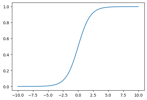
if y_range is not None: _layers.append(SigmoidRange(*y_range))_layers[LinBnDrop(
(0): Linear(in_features=11, out_features=200, bias=True)
(1): ReLU(inplace=True)
),
LinBnDrop(
(0): Linear(in_features=200, out_features=100, bias=True)
(1): ReLU(inplace=True)
),
LinBnDrop(
(0): Linear(in_features=100, out_features=1, bias=True)
),
fastai.layers.SigmoidRange(low=0, high=1)]self.layers
self.layers = nn.Sequential(*_layers)
The final piece to handling the layers in the model is to wrap them in a nn.Sequential model, so that inputs are passed sequentially to each layer in the list _layers.
layers = nn.Sequential(*_layers)
layers
Sequential(
(0): LinBnDrop(
(0): Linear(in_features=11, out_features=200, bias=True)
(1): ReLU(inplace=True)
)
(1): LinBnDrop(
(0): Linear(in_features=200, out_features=100, bias=True)
(1): ReLU(inplace=True)
)
(2): LinBnDrop(
(0): Linear(in_features=100, out_features=1, bias=True)
)
(3): fastai.layers.SigmoidRange(low=0, high=1)
)forward
if self.n_emb != 0:
In this example, n_emb is not equal to 0 so the following code will run.
x = [e(x_cat[:,i]) for i,e in enumerate(self.embeds)]
In this line of code, the categorical variable columns are passed to the corresponding Embedding and the output tensor is stored in a list.
x = [e(x_cat[:,i]) for i,e in enumerate(embeds)]
len(x), len(x[0]), len(x[1])
(2, 10, 10)There are 10 rows in x_cat. The Embedding corresponding to the first column outputs 2 columns of tensors, and the Embedding corresponding to the second column outputs 8 columns of tensors.
x[0].shapetorch.Size([10, 2])x[1].shapetorch.Size([10, 8])The following line takes the list of tensors x (with a 10 x 2 and 10 x 8 tensor) and concatenates them into a single 10 x 10 tensor.
x = torch.cat(x, 1)
x = torch.cat(x,1)x.shapetorch.Size([10, 10])xtensor([[ 1.3314e-03, 8.6398e-03, 2.0744e-04, 2.5392e-03, 9.3644e-03,
7.1224e-03, -3.1766e-04, 1.0164e-03, 1.3433e-02, 7.1327e-03],
[-1.0157e-02, -8.8875e-03, -1.5988e-02, -1.0913e-03, 7.1520e-03,
3.9139e-04, 1.3059e-02, 2.4659e-03, -1.9776e-02, 1.7896e-04],
[-4.9903e-04, 5.2634e-03, 3.7818e-03, 7.0511e-03, -1.7237e-02,
-8.4348e-03, 4.3514e-03, 2.6589e-03, -5.8710e-03, 8.2689e-04],
[ 1.3314e-03, 8.6398e-03, -1.5988e-02, -1.0913e-03, 7.1520e-03,
3.9139e-04, 1.3059e-02, 2.4659e-03, -1.9776e-02, 1.7896e-04],
[ 1.3314e-03, 8.6398e-03, -7.1988e-04, -9.0609e-03, -4.8712e-04,
-1.0811e-02, 1.7623e-04, 7.8226e-04, 1.9316e-03, 4.0967e-03],
[-1.0157e-02, -8.8875e-03, 1.2554e-02, -7.1496e-03, 8.5392e-03,
5.1299e-03, 5.3973e-03, 5.6551e-03, 5.0579e-03, 2.2245e-03],
[-4.9903e-04, 5.2634e-03, -6.8548e-03, 5.6356e-03, -1.5072e-02,
-1.6107e-02, -1.4790e-02, 4.3227e-03, -1.2503e-03, 7.8212e-03],
[-4.9903e-04, 5.2634e-03, 4.0380e-03, -7.1398e-03, 8.3373e-03,
-9.5855e-03, 4.5363e-03, 1.2461e-02, -3.0651e-03, -1.2869e-02],
[ 1.3314e-03, 8.6398e-03, 1.2554e-02, -7.1496e-03, 8.5392e-03,
5.1299e-03, 5.3973e-03, 5.6551e-03, 5.0579e-03, 2.2245e-03],
[-8.4988e-05, 7.2906e-03, -6.8548e-03, 5.6356e-03, -1.5072e-02,
-1.6107e-02, -1.4790e-02, 4.3227e-03, -1.2503e-03, 7.8212e-03]],
grad_fn=<CatBackward0>)The following line of code passes the x tensor through the nn.Dropout function. If I understand correctly, since I defined embed_p as 0, passing it through the Dropout layer will not affect the tensor x.
x = self.emb_drop(x)
x = emb_drop(x)if self.n_cont != 0
In this example, n_cont is not 0 so the following code will run.
Since bn_cont is None, the code x_cont = self.bn_cont(x_cont) will not run.
if self.bn_cont is not None: x_cont = self.bn_cont(x_cont)
if bn_cont is not None: x_cont = bn_cont(x_cont)In the following line, if n_emb is not 0, it will concatenate x (which holds the outputs of the categorical Embeddings) with x_cont (which holds the continuous variable columns) into a single tensor. If n_emb is 0, it will assign x_cont to x.
In this example, n_emb is not 0 so it will concatenate x with x_cont.
x = torch.cat([x, x_cont], 1) if self.n_emb != 0 else x_cont
x.shapetorch.Size([10, 10])x = torch.cat([x, x_cont], 1) if n_emb != 0 else x_contThe concatenation has added a column of tensors (continuous variable) to x:
x.shapetorch.Size([10, 11])return
The final piece of the forward method is to return the outputs of the model. This is done by passing our 11 inputs in x (10 categorical embeddings, 1 continuous variable) to the layers nn.Sequential model defined before.
self.layers(x)
layersSequential(
(0): LinBnDrop(
(0): Linear(in_features=11, out_features=200, bias=True)
(1): ReLU(inplace=True)
)
(1): LinBnDrop(
(0): Linear(in_features=200, out_features=100, bias=True)
(1): ReLU(inplace=True)
)
(2): LinBnDrop(
(0): Linear(in_features=100, out_features=1, bias=True)
)
(3): fastai.layers.SigmoidRange(low=0, high=1)
)The output is a tensor with 10 values, 1 for each of the 10 input rows.
layers(x)tensor([[0.5217],
[0.5210],
[0.5216],
[0.5214],
[0.5149],
[0.5192],
[0.5377],
[0.5174],
[0.5223],
[0.5221]], grad_fn=<AddBackward0>)Final Thoughts
I really enjoyed this exercise and will definitely apply the same process of running line-by-line code in the future when I am trying to understand fastai (or other) library source code. By the end of this exercise, I was surprised at how simple and straightforward it is to build a TabularModel object. It’s so powerful given its simplicity.
I hope you enjoyed this blog post!