Training Collaborative Filtering Models on MovieLens 100k with Different Weight Decay Values

machine learning

fastai

python

In this notebook I explore the question—how does the wd (weight decay) parameter affect model performance and weight distributions? I use the MovieLens 100k subset as the dataset.

Author

Vishal Bakshi

Published

June 3, 2024

Background

In fastai Part 1 Lesson 7 (Chapter 8 of the textbook), we are introduced to the concept of weight decay, where the sum of the squared weights multiplied by a factor wd is added to the loss. In practice, instead of adding wd times the sum of squared weights to the loss (which would result in a large values of loss which destabilizes training), we add the derivative of that to the parameters’ gradients. In pseudo code:

for param in model.parameters():
  param.grad += wd * sum(params)

By increasing the loss with the squared sum of weights, we are forcing the model to minimize the weights when it minimizes the loss, which makes the model generalize better (as large weights result in a neural net function with sharp peaks and troughs that can overfit to the training data).

In this notebook I’ll train on the MovieLens 100k dataset using different values of weight decay and then plotting both the resulting training and validation loss curves and weight distribution to see how weight decay affects the training process and the resulting model.

Create `DataLoaders` and `Learner`

I’l re-use the code from Chapter 8 to create DataLoaders and the Learner.

from fastai.collab import *
from fastai.tabular.all import *
path = untar_data(URLs.ML_100k)

100.15% [4931584/4924029 00:01<00:00]

ratings = pd.read_csv(path/'u.data', delimiter='\t', header=None, names=['user', 'movie', 'rating', 'timestamp'])
ratings.head()

	user	movie	rating	timestamp
0	196	242	3	881250949
1	186	302	3	891717742
2	22	377	1	878887116
3	244	51	2	880606923
4	166	346	1	886397596

movies = pd.read_csv(path/'u.item', delimiter='|', encoding='latin-1', usecols=(0,1), names=('movie', 'title'), header=None)
movies.head()

	movie	title
0	1	Toy Story (1995)
1	2	GoldenEye (1995)
2	3	Four Rooms (1995)
3	4	Get Shorty (1995)
4	5	Copycat (1995)

ratings = ratings.merge(movies)
ratings.head()

	user	movie	rating	timestamp	title
0	196	242	3	881250949	Kolya (1996)
1	63	242	3	875747190	Kolya (1996)
2	226	242	5	883888671	Kolya (1996)
3	154	242	3	879138235	Kolya (1996)
4	306	242	5	876503793	Kolya (1996)

dls = CollabDataLoaders.from_df(ratings, item_name='title', bs=64)
dls.show_batch()

	user	title	rating
0	294	Money Talks (1997)	3
1	486	Crossing Guard, The (1995)	4
2	13	High Noon (1952)	5
3	878	My Life as a Dog (Mitt liv som hund) (1985)	5
4	433	Star Wars (1977)	5
5	847	Streetcar Named Desire, A (1951)	3
6	833	Akira (1988)	4
7	503	Englishman Who Went Up a Hill, But Came Down a Mountain, The (1995)	3
8	5	Last of the Mohicans, The (1992)	1
9	868	Stand by Me (1986)	4

In the text, the following Learner resulted in the lowest validation loss (0.821688) so I’ll just use that in this experiment.

learn = collab_learner(dls, n_factors=50, y_range=(0, 5.5))

I’ll do an initial training to sort my head around how I’m going to collect data during the experiment.

learn.fit_one_cycle(5, 5e-3, wd=0.1)

epoch	train_loss	valid_loss	time
0	0.882671	0.955993	00:12
1	0.654915	0.892832	00:12
2	0.525330	0.872967	00:12
3	0.436863	0.858952	00:12
4	0.438653	0.854505	00:12

Planning the Experiment

I’ll be trying that same learning process (5 epochs, 5e-3 learning rate) with different weight decay wd values (from 0.0001 to 1.0). Once the experiment is done, I want to visualize the following for all wd values:

training loss curve .
validation loss curve.
distribution of model parameters.

I’ll reference the plot_loss source code for how to capture those values from the Learner’s Recorder object.

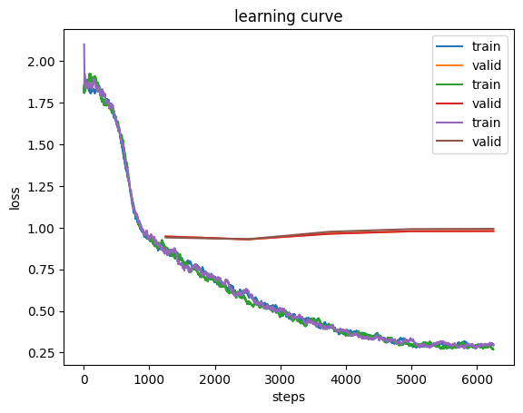
But first, I’ll plot the losses using that plot_loss function to have a baseline reference:

learn.recorder.plot_loss();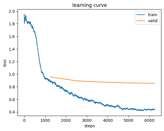

Plotting Loss Values

The following line in plot_loss plots the training loss:

ax.plot(list(range(skip_start, len(self.losses))), self.losses[skip_start:], label='train')

I’ll see if I can recreate that plot:

ax=plt.gca()
ax.plot(list(range(5, len(learn.recorder.losses))), learn.recorder.losses[5:], label='train');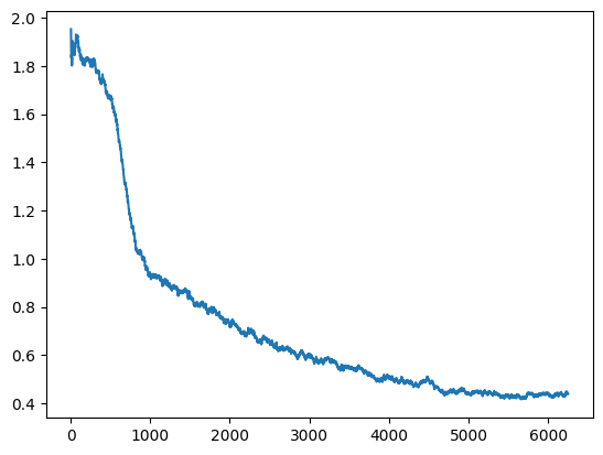

Cool, that looks the same! Now for the validation loss:

ax=plt.gca()
ax.plot(list(range(5, len(learn.recorder.losses))), learn.recorder.losses[5:], label='train');
idx = (np.array(learn.recorder.iters)<5).sum()
valid_col = learn.recorder.metric_names.index('valid_loss') - 1
ax.plot(learn.recorder.iters[idx:], L(learn.recorder.values[idx:]).itemgot(valid_col), label='valid')
ax.legend();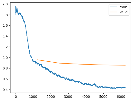

Nice, I’m able to recreate plot_loss using the raw data recorded in the Recorder.

Plotting Distribution of Weights

Next, I want to be able to visualize (and calculate summary statistics for) the weights of the model.

The model has four sets of parameters: the user and item weights, and the user and item biases.

learn.model

EmbeddingDotBias(
  (u_weight): Embedding(944, 50)
  (i_weight): Embedding(1665, 50)
  (u_bias): Embedding(944, 1)
  (i_bias): Embedding(1665, 1)
)

for p in learn.model.parameters():
  print(p.shape)

torch.Size([944, 50])
torch.Size([1665, 50])
torch.Size([944, 1])
torch.Size([1665, 1])

Let’s take a look at the first set of parameters, which are the u_weight (user weight) parameters. This is the embedding with 50 latent factors for each user.

pd.Series(first(learn.model.parameters()).flatten().detach().numpy()).hist();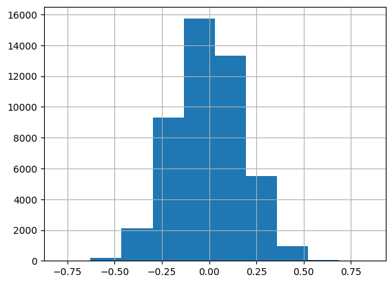

Next, let’s look at the bias parameters for the users (u_bias):

u_bias_params = next(itertools.islice(learn.model.parameters(), 2, None))

u_bias_params.shape

torch.Size([944, 1])

pd.Series(u_bias_params.flatten().detach().numpy()).hist();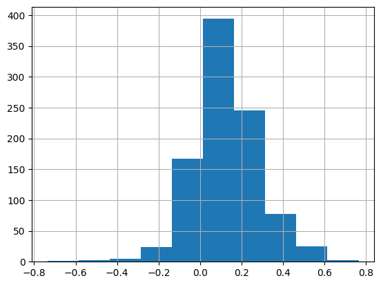

Looking at all of the parameters:

torch.nn.utils.parameters_to_vector(learn.model.parameters()).shape, 944*50 + 944*1 + 1665*50 + 1665*1

(torch.Size([133059]), 133059)

pd.Series(torch.nn.utils.parameters_to_vector(learn.model.parameters()).detach().numpy()).hist();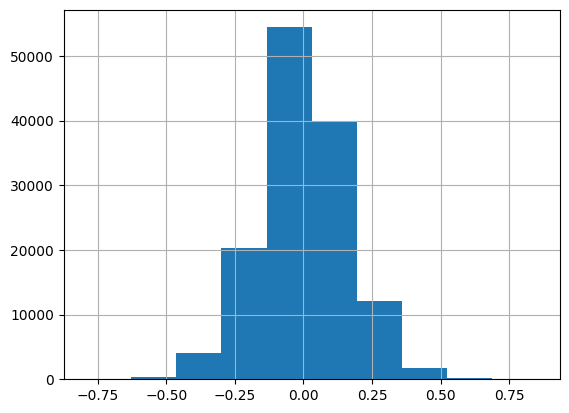

Now I know how to access and plot the training loss, validation loss and model weights.

Estimating Runtime and Storage Size

Each model takes about 1 minute to run on Colab. I trained on Paperspace CPUs but it was taking 30+ seconds per epoch (while it takes 10-14 seconds on Colab). I have a 2015 Mac so I can’t install fastai locally (if I’m interpreting this note correctly).

Originally I was going to use torch.arange to create weight decay values (without subtracting 1e-6 from the upper bound as I eventually did below), but it acculumated floating point error. The following tensor should stop at 0.0990 but goes up to 0.1000 because of floating point error.

torch.arange(0.01, 0.1, 0.001)

tensor([0.0100, 0.0110, 0.0120, 0.0130, 0.0140, 0.0150, 0.0160, 0.0170, 0.0180,
        0.0190, 0.0200, 0.0210, 0.0220, 0.0230, 0.0240, 0.0250, 0.0260, 0.0270,
        0.0280, 0.0290, 0.0300, 0.0310, 0.0320, 0.0330, 0.0340, 0.0350, 0.0360,
        0.0370, 0.0380, 0.0390, 0.0400, 0.0410, 0.0420, 0.0430, 0.0440, 0.0450,
        0.0460, 0.0470, 0.0480, 0.0490, 0.0500, 0.0510, 0.0520, 0.0530, 0.0540,
        0.0550, 0.0560, 0.0570, 0.0580, 0.0590, 0.0600, 0.0610, 0.0620, 0.0630,
        0.0640, 0.0650, 0.0660, 0.0670, 0.0680, 0.0690, 0.0700, 0.0710, 0.0720,
        0.0730, 0.0740, 0.0750, 0.0760, 0.0770, 0.0780, 0.0790, 0.0800, 0.0810,
        0.0820, 0.0830, 0.0840, 0.0850, 0.0860, 0.0870, 0.0880, 0.0890, 0.0900,
        0.0910, 0.0920, 0.0930, 0.0940, 0.0950, 0.0960, 0.0970, 0.0980, 0.0990,
        0.1000])

The following arange call results in the correct number of values:

torch.arange(0.0001, 0.001-1e-6, 0.00001).shape, \
torch.arange(0.001, 0.01-1e-6, 0.0001).shape, \
torch.arange(0.01, 0.10-1e-6, 0.001).shape, \
torch.arange(0.1, 1.0-1e-6, 0.01).shape

(torch.Size([90]), torch.Size([90]), torch.Size([90]), torch.Size([90]))

wds = torch.cat([
    torch.arange(0.0001, 0.001-1e-6, 0.00001),
    torch.arange(0.001, 0.01-1e-6, 0.0001),
    torch.arange(0.01, 0.10-1e-6, 0.001),
    torch.arange(0.1, 1.0-1e-6, 0.01)])

wds.shape

torch.Size([360])

pd.Series(wds).plot();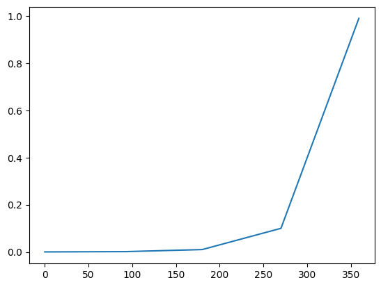

Next, I’ll estimate the disk space required to store the training loss, validation loss and weights for all 360 models (1 per wd value).

With ChatGPT’s help:

import pickle
import io

def get_pickled_object_size(obj):
    # Create a BytesIO buffer
    buffer = io.BytesIO()
    # Pickle the object into the buffer
    pickle.dump(obj, buffer)
    # Get the size of the buffer
    size = buffer.getbuffer().nbytes
    return size

res = {
    'training_loss': learn.recorder.losses,
    'iters': learn.recorder.iters,
    'valid_cols': learn.recorder.metric_names.index('valid_loss') - 1,
    'validation_loss': L(learn.recorder.values[(np.array(learn.recorder.iters)<5).sum():]).itemgot(learn.recorder.metric_names.index('valid_loss') - 1),
    'weights': torch.nn.utils.parameters_to_vector(learn.model.parameters())
}

size = get_pickled_object_size(res)
print(f'The size of the pickled object for one model is {size/1e6} MB.')
print(f'The total size of the pickled objects for 360 models will be ~{360*size/1e6} MB.')

The size of the pickled object for one model is 2.345662 MB.
The total size of the pickled objects for 360 models will be ~844.43832 MB.

That’s quite a bit. And seem unnecessarily large. learn.recorder.losses is a list of tensors:

learn.recorder.losses[:5]

[TensorBase(1.8254),
 TensorBase(1.8496),
 TensorBase(1.9542),
 TensorBase(1.8464),
 TensorBase(1.9200)]

Perhaps I can convert that to a list of floats and see if it reduces the storage size:

res = {
    'training_loss': [t.item() for t in learn.recorder.losses],
    'iters': learn.recorder.iters,
    'valid_cols': learn.recorder.metric_names.index('valid_loss') - 1,
    'validation_loss': L(learn.recorder.values[(np.array(learn.recorder.iters)<5).sum():]).itemgot(learn.recorder.metric_names.index('valid_loss') - 1),
    'weights': torch.nn.utils.parameters_to_vector(learn.model.parameters())
}

size = get_pickled_object_size(res)
print(f'The size of the pickled object for one model is {size/1e6} MB.')
print(f'The total size of the pickled objects for 360 models will be ~{360*size/1e6} MB.')

The size of the pickled object for one model is 0.589096 MB.
The total size of the pickled objects for 360 models will be ~212.07456 MB.

That’s better! Most of the size is coming from my weights.

size = get_pickled_object_size(torch.nn.utils.parameters_to_vector(learn.model.parameters()))
print(f'The size of the pickled object for one model is {size/1e6} MB.')
print(f'The total size of the pickled objects for 360 models will be ~{360*size/1e6} MB.')

The size of the pickled object for one model is 0.532648 MB.
The total size of the pickled objects for 360 models will be ~191.75328 MB.

With ChatGPT’s help: there are 133059 float32 elements in the weights tensor. Each float32 element is 4 bytes large. 4 x 133059 is 532236 bytes, which is ~0.5MB. I’ll keep them as float32’s and accept the larger disk space (since I’m keeping this only temporarily).

Running the Experiment

Now I can run the experiment and collect the data on it. I’ll do a quick run with 3 models and save the Learner objects to make sure I’m collecting data correctly.

res = {'training_loss': [], 'iters': [], 'validation_loss': [], 'weights': []}
learners = []
count = 0

for wd in wds:
  if count == 3: break
  learn = collab_learner(dls, n_factors=50, y_range=(0, 5.5))
  learn.fit_one_cycle(5, 5e-3, wd=wd.item())
  learn.recorder.plot_loss();
  learners.append(learn)

  res['training_loss'].append([t.item() for t in learn.recorder.losses])
  res['iters'].append(learn.recorder.iters)
  res['validation_loss'].append(L(learn.recorder.values[(np.array(learn.recorder.iters)<5).sum():]).itemgot(learn.recorder.metric_names.index('valid_loss') - 1))
  res['weights'].append(torch.nn.utils.parameters_to_vector(learn.model.parameters()))
  count += 1

epoch	train_loss	valid_loss	time
0	0.867206	0.947485	00:12
1	0.612190	0.929238	00:12
2	0.401040	0.964420	00:13
3	0.298337	0.977934	00:12
4	0.293123	0.979958	00:12

epoch	train_loss	valid_loss	time
0	0.879830	0.946919	00:12
1	0.544347	0.930262	00:12
2	0.416691	0.962877	00:12
3	0.298801	0.978486	00:12
4	0.269458	0.979087	00:11

epoch	train_loss	valid_loss	time
0	0.867352	0.940780	00:11
1	0.624375	0.930750	00:12
2	0.405802	0.975494	00:12
3	0.325339	0.991441	00:12
4	0.300811	0.993090	00:12

Good to know—it plots on the same chart! I could just use this functionality instead of saving the training and validation loss values, but I want to keep those to do additional visualizations.

Next, I’ll check that the recorded values are the same as the Learner object.

len(res['training_loss'])

res['training_loss'][0] == [t.item() for t in learners[0].recorder.losses], \
res['iters'][1] == learners[1].recorder.iters, \
res['validation_loss'][2] == L(learners[2].recorder.values[(np.array(learners[2].recorder.iters)<5).sum():]).itemgot(learners[2].recorder.metric_names.index('valid_loss') - 1), \
(res['weights'][2] == torch.nn.utils.parameters_to_vector(learners[2].model.parameters())).sum()

(True, True, True, tensor(133059))

Testing that I can pickle and unpickle the results:

save_pickle('wd_res_test.pkl', res)
res = load_pickle('/content/wd_res_test.pkl')

res['training_loss'][0] == [t.item() for t in learners[0].recorder.losses], \
res['iters'][1] == learners[1].recorder.iters, \
res['validation_loss'][2] == L(learners[2].recorder.values[(np.array(learners[2].recorder.iters)<5).sum():]).itemgot(learners[2].recorder.metric_names.index('valid_loss') - 1), \
(res['weights'][2] == torch.nn.utils.parameters_to_vector(learners[2].model.parameters())).sum()

(True, True, True, tensor(133059))

Nice!

However, I noticed that some epochs took up to 13 seconds. I wonder if training time is affected by weight decay value? I’ll train with a much larger weight decay and see if it speeds up the training.

learn = collab_learner(dls, n_factors=50, y_range=(0, 5.5))
learn.fit_one_cycle(5, 5e-3, wd=0.9)

epoch	train_loss	valid_loss	time
0	0.990363	1.074203	00:12
1	1.003346	1.067053	00:12
2	0.976281	1.029760	00:12
3	0.978760	1.001970	00:12
4	0.912565	0.993564	00:12

Nope, seems like the training time per epoch just varies.

res = {'wds': wds, 'training_loss': [], 'iters': [], 'validation_loss': [], 'weights': []}

for wd in wds:
  learn = collab_learner(dls, n_factors=50, y_range=(0, 5.5))
  with learn.no_logging(), learn.no_bar():
    learn.fit_one_cycle(5, 5e-3, wd=wd.item())

  res['training_loss'].append([t.item() for t in learn.recorder.losses])
  res['iters'].append(learn.recorder.iters)
  res['validation_loss'].append(L(learn.recorder.values[(np.array(learn.recorder.iters)<5).sum():]).itemgot(learn.recorder.metric_names.index('valid_loss') - 1))
  res['weights'].append(torch.nn.utils.parameters_to_vector(learn.model.parameters()))

save_pickle('wd_res.pkl', res)

Analyzing Training Results

`matplotlib` Animations

I’ll create an animation with matplotlib which highlights the training loss curve for each weight decay value and prints the weight decay value on the plot.

To start, I’ll make sure that all 360 of my training loss lists are of the same length (6250 steps).

#wd_res = load_pickle('/content/wd_res.pkl')

trn_loss_t = torch.stack([torch.tensor(el) for el in wd_res['training_loss']])

trn_loss_t.shape # looks good

torch.Size([360, 6250])

Next, I’ll create my x values for the plot as a range from 0 to 6249.

x = list(range(len(wd_res['training_loss'][0])))
len(x), x[:5], x[-5:]

(6250, [0, 1, 2, 3, 4], [6245, 6246, 6247, 6248, 6249])

With ChatGPT’s help, I used the following code to create an animated GIF which highlights the training and validation loss curves for the given weight decay value.

Show the code

import numpy as np
import matplotlib.pyplot as plt
from matplotlib.animation import FuncAnimation, PillowWriter

# Prepare Data
x = list(range(len(wd_res['training_loss'][0])))

data = wd_res['training_loss']

labels = wd_res['wds']

# Create Static Plot
fig, ax = plt.subplots()
ax.set_xlabel('Step')
ax.set_ylabel('Training Loss')

lines = [ax.plot(x, y, alpha=0.0, color='#ff0088', linewidth=2)[0] for y in data]  # Initial lines with lower opacity
text = ax.text(0.5, 1.05, "", transform=ax.transAxes, ha="center")

# Define Animation Function
def animate(i):
    # Reset all lines to low opacity
    for line in lines:
        line.set_alpha(0.0)

    # Highlight the current line
    lines[i].set_alpha(1.0)

    # Update the text
    text.set_text(f"weight decay = {labels[i].item():.5f}")

    return lines + [text]

# Create Animation
ani = FuncAnimation(fig, animate, frames=len(data), interval=150, blit=True)

# Save as GIF
gif_writer = PillowWriter(fps=6)
ani.save('training_loss.gif', writer=gif_writer)

Here’s the GIF for training loss. The loss curve slowly moves upward with the minimum loss value increasing as weight decay increases. It really starts picking up at a weight decay value of around 0.1.

Here’s the GIF for the validation loss—the loss curve starts out decreasing first then increasing and at a weight decay value of around 0.03, starts decreasing monotonically with the minimum loss reaching its minimum. It starts to shift upwards again at around a loss of 0.3.

Next, I’ll animate the distribution of the weights (as weight decay value changes), modifying the above code accordingly:

Show the code

import numpy as np
import matplotlib.pyplot as plt
from matplotlib.animation import FuncAnimation, PillowWriter

# Prepare Data
data = wd_res['weights']
labels = wd_res['wds']

# Create Static Plot
fig, ax = plt.subplots()
ax.set_xlabel('Weights')
ax.set_ylabel('Count')

# Define Animation Function
def animate(i):
    ax.clear()  # Clear previous histogram
    n, bins, patches = ax.hist(data[i].detach().numpy())
    ax.set_title(f"weight decay = {labels[i].item():.5f}")
    ax.set_xlabel('Weights')
    ax.set_ylabel('Count')
    ax.set_xlim(-0.5, 0.5)  # Set x-axis limits to keep consistent across frames
    ax.set_ylim(0, 75000)  # Set y-axis limits to keep consistent across frames
    return patches

# Create Animation
ani = FuncAnimation(fig, animate, frames=len(data), interval=150, blit=True)

# Save as GIF
gif_writer = PillowWriter(fps=6)
ani.save('weights.gif', writer=gif_writer)

Here’s the resulting GIF showing the changing distribution of weights. Note that the range of weights starts out beyond -0.5 to 0.5, and ends up within -0.2 and +0.2 as the weight decay value increases to 1.0.

Trends

I’ll next look at how the final training loss, validation loss and median weight value changes with weight decay values.

min_trn_loss = trn_loss_t.min(dim=-1)[0]
min_trn_loss.shape

torch.Size([360])

Show the code

plt.scatter(wd_res['wds'], min_trn_loss, s=5, alpha=0.4)

# Set axis labels
plt.xlabel('Weight Decay Value')
plt.ylabel('Minimum Training Loss')

# Display the plot
plt.show();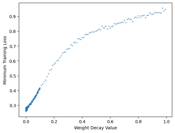

As the weight-decay value increases, so does the training loss.

val_loss_t = torch.stack([torch.tensor(el) for el in wd_res['validation_loss']])
min_val_loss = val_loss_t.min(dim=-1)[0]
min_val_loss.shape

torch.Size([360])

Show the code

plt.scatter(wd_res['wds'], min_val_loss, s=5, alpha=0.4)

# Set axis labels
plt.xlabel('Weight Decay Value')
plt.ylabel('Minimum Validation Loss')

# Display the plot
plt.show();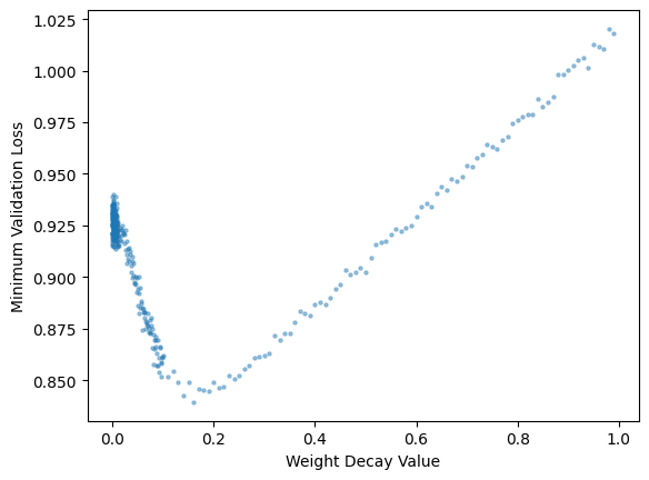

The minimum validation loss achieved during training reaches a minimum at a weight decay value of around 0.2 and then increases as weight decay increases to 1.0.

weights_t = torch.stack([el.clone().detach() for el in wd_res['weights']])
weights_t.shape

torch.Size([360, 133059])

med_weights_t = weights_t.median(dim=-1)[0]
med_weights_t.shape

torch.Size([360])

Show the code

plt.scatter(wd_res['wds'], med_weights_t, s=5, alpha=0.4)

# Set axis labels
plt.xlabel('Weight Decay Value')
plt.ylabel('Median Weight Value')

# Display the plot
plt.show();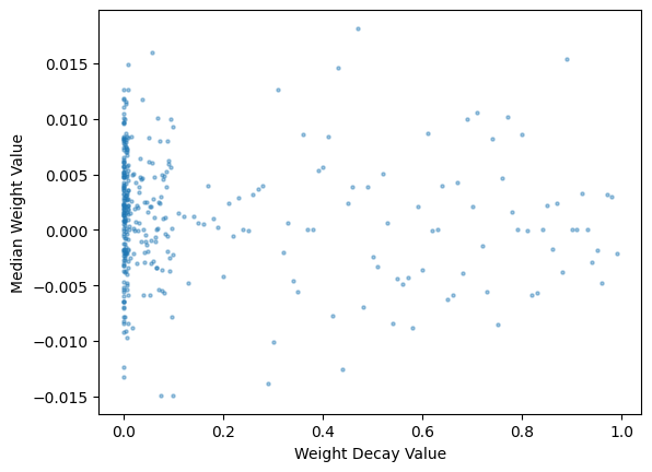

It’s a bit difficult to see trends from this chart, but the but median weights generally seem to be decreasing as weight decay value increaeses–although there is a considerable amount of variability.

mean_weights_t = weights_t.mean(dim=-1)
mean_weights_t.shape

torch.Size([360])

Show the code

plt.scatter(wd_res['wds'], mean_weights_t, s=5, alpha=0.4)

# Set axis labels
plt.xlabel('Weight Decay Value')
plt.ylabel('Mean Weight Value')

# Display the plot
plt.show();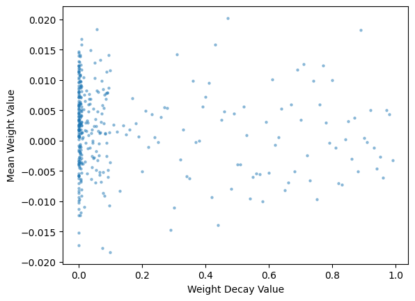

The mean weights follow a similar trend—generally narrowing in range as weight decay value increases. I’ll look at the absolute value of mean and median and see if any trends appear:

abs_med_weights_t = weights_t.abs().median(dim=-1)[0]
abs_med_weights_t.shape

torch.Size([360])

Show the code

plt.scatter(wd_res['wds'], abs_med_weights_t, s=5, alpha=0.4)

# Set axis labels
plt.xlabel('Weight Decay Value')
plt.ylabel('Median Absolute Weight Value')

# Display the plot
plt.show();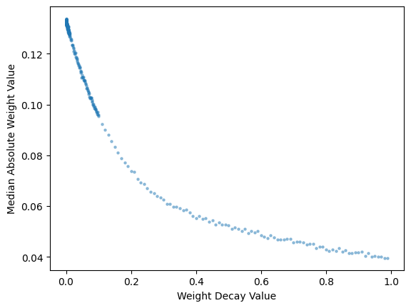

That’s much clearer! the median absolute value of the weights exponentially decreases as the weight decay value increases. I’ll look at the mean absolute value we well:

abs_mean_weights_t = weights_t.abs().mean(dim=-1)
abs_mean_weights_t.shape

torch.Size([360])

Show the code

plt.scatter(wd_res['wds'], abs_mean_weights_t, s=5, alpha=0.4)

# Set axis labels
plt.xlabel('Weight Decay Value')
plt.ylabel('Mean Absolute Weight Value')

# Display the plot
plt.show();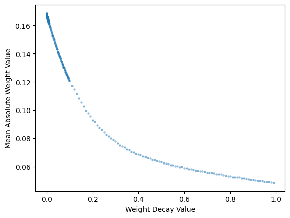

Yup! The mean absolute value of the weights exponentially decreases as well (as weight decay value goes to 1.0).

Final Thoughts

As always, I love experimenting with (relatively) simple concepts and observing how they affect training performance and results. Recapping the trends I observed:

Minimum training loss increases as weight decay increases.
Minimum validation loss decreases until a point (for this dataset and model, until a weight decay value of ~0.2) and then increases as weight decay increases.
The mean and median absolute values of the final weights decreases (exponentially) as weight decay increases.

I also enjoyed creating animated GIFs as a visual tool to illustrate the distributions and trends of weights and losses as weight decay increases. The resulting GIFs could be improved by tweaking frame rate and other parameters, but I’m happy with the overall trends they convey, which match the static plots I created.

As always, I hope you enjoyed this blog post! Follow me on Twitter @vishal_learner.

Background

Create DataLoaders and Learner

Planning the Experiment

Plotting Loss Values

Plotting Distribution of Weights

Estimating Runtime and Storage Size

Running the Experiment

Analyzing Training Results

matplotlib Animations

Trends

Final Thoughts

Create `DataLoaders` and `Learner`

`matplotlib` Animations