Training a Collaborative Filtering Model Using Cross Entropy Loss

In this notebook I create a collaborative filtering (classifier) architecture suited to use with cross-entropy loss.

Background

In this notebook, I’ll work through the following prompt given in the “Further Research” of Chapter 8 (Collaborative Filtering):

Create a model for MovieLens that works with cross-entropy loss, and compare it to the model in this chapter.

Visual Inspection

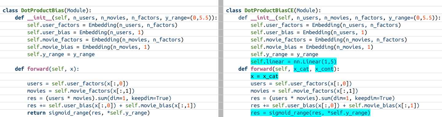
I’ll start by visually inspecting the DotProductBias model from the chapter that outputs one prediction and a DotProductBiasCE model that I’ve written to output 5 predictions (so that it works with Cross Entropy loss).

Visual inspection of DotProductBias Modules

Creating DataLoaders

Since I want to use Cross Entropy loss, I’ll need to specify that the outputs (or targets) are discrete categories and not continuous numbers. To do this, I’ll use TabularDataLoaders.

from fastai.collab import *
from fastai.tabular.all import *
path = untar_data(URLs.ML_100k)

100.15% [4931584/4924029 00:00<00:00]

ratings = pd.read_csv(path/'u.data', delimiter='\t', header=None, names=['user', 'movie', 'rating', 'timestamp'])
movies = pd.read_csv(path/'u.item', delimiter='|', encoding='latin-1', usecols=(0,1), names=('movie', 'title'), header=None)
ratings = ratings.merge(movies)
ratings.head()

	user	movie	rating	timestamp	title
0	196	242	3	881250949	Kolya (1996)
1	63	242	3	875747190	Kolya (1996)
2	226	242	5	883888671	Kolya (1996)
3	154	242	3	879138235	Kolya (1996)
4	306	242	5	876503793	Kolya (1996)

dls = TabularDataLoaders.from_df(
    ratings[['user', 'title', 'rating']],
    procs=[Categorify],
    cat_names=['user','title'],
    y_names=['rating'],
    y_block=CategoryBlock)

TabularDataLoaders will provide three elements for each training item: the categorical inputs, the continuous inputs and the outputs (or targets, or dependent variable):

b = dls.one_batch()
len(b), b[0].shape, b[1].shape, b[2].shape

(3, torch.Size([64, 2]), torch.Size([64, 0]), torch.Size([64, 1]))

This is important to note before I create the model since the forward pass will receive two values: x_cat (categorical inputs) and x_cont (continuous inputs).

The TabularDataLoaders also has a vocabulary—the five possible values for the dependent variable (1 through 5).

dls.vocab

[1, 2, 3, 4, 5]

Creating the New Model

I’ll start by creating the original DotProductBias model for reference:

class DotProductBias(Module):
  def __init__(self, n_users, n_movies, n_factors, y_range=(0,5.5)):
    self.user_factors = Embedding(n_users, n_factors)
    self.user_bias = Embedding(n_users, 1)
    self.movie_factors = Embedding(n_movies, n_factors)
    self.movie_bias = Embedding(n_movies, 1)
    self.y_range = y_range

  def forward(self, x):
    users = self.user_factors(x[:,0])
    movies = self.movie_factors(x[:,1])
    res = (users * movies).sum(dim=1, keepdim=True)
    res += self.user_bias(x[:,0]) + self.movie_bias(x[:,1])
    return sigmoid_range(res, *self.y_range)

The biggest change in the behavior of the model, to allow the usage of Cross Entropy loss, is to make it output 5 activations instead of 1. I’ll do so by passing the dot product through an nn.Linear layer that projects that value into 5 dimensions (one for each rating 1-5) in the forward pass.

The second change in the model behavior is to allow two inputs in the forward pass: x_cat for categorical variables and x_cont for continuous variables, which is how TabularDataLoaders prepares the data. In the case of the MovieLens 100k subset, there are no continuous variables. The only variables of interest are the categoricals users and movies, one column for each in the input x_cat.

class DotProductBiasCE(Module):
  def __init__(self, n_users, n_movies, n_factors, y_range=(0,5.5)):
    self.user_factors = Embedding(n_users, n_factors)
    self.user_bias = Embedding(n_users, 1)
    self.movie_factors = Embedding(n_movies, n_factors)
    self.movie_bias = Embedding(n_movies, 1)
    self.y_range = y_range
    self.linear = nn.Linear(1, 5)

  def forward(self, x_cat, x_cont):
    x = x_cat
    users = self.user_factors(x[:,0])
    movies = self.movie_factors(x[:,1])
    res = (users * movies).sum(dim=1, keepdim=True)
    res += self.user_bias(x[:,0]) + self.movie_bias(x[:,1])
    res = sigmoid_range(res, *self.y_range)
    return self.linear(res)

n_users = len(dls.classes['user'])
n_movies = len(dls.classes['title'])

n_users, n_movies

(944, 1665)

model = DotProductBiasCE(n_users, n_movies, 50)

model(x_cat=b[0], x_cont=b[1]).shape

torch.Size([64, 5])

Training the Model

I’ll use the same hyperparameters (5 epochs, LR=5e-3 and weight decay of 0.1) as the best training run in the text. Of course, this is a different model so these values may not be optimal.

model = DotProductBiasCE(n_users, n_movies, n_factors=50)
learn = Learner(dls, model, loss_func=CrossEntropyLossFlat(), metrics=accuracy)

learn.fit_one_cycle(5, 5e-3, wd=0.1)

epoch	train_loss	valid_loss	accuracy	time
0	1.426626	1.445451	0.337150	00:15
1	1.281385	1.425528	0.339900	00:15
2	1.171326	1.431534	0.364500	00:16
3	1.105676	1.438475	0.361650	00:16
4	1.127306	1.438119	0.363450	00:14

The model’s not great (although it’s better than guessing ratings randomly which would have an accuracy of 20%) and it’s difficult to compare it with the DotProductBias model since that model only measured RMSE and not accuracy.

I’ll take a look at the predictions and see how they compare to the actual ratings.

Looking at the confusion matrix below, here are some observations:

• The model did not predict any 5s.
• The best predicted rating was a 4 (with 4327/6692, or 65% correct predictions).
• Most of the model’s predictions are 3s or 4s.

interp = ClassificationInterpretation.from_learner(learn)
interp.plot_confusion_matrix()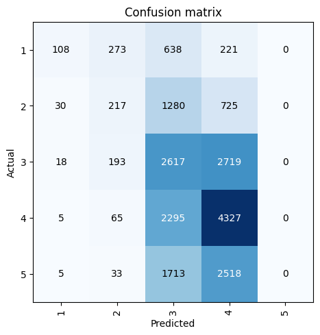

Improving the Model

Looking at these results, I’m starting to think that using sigmoid_range in this model is causing it to predict values in the middle of the range (2-4) and making it harder for it to predict ratings that are at the edges (1 and 5). I’ll remove y_range and sigmoid_range from the model and train it again to see if it makes a difference.

class DotProductBiasCE(Module):
  def __init__(self, n_users, n_movies, n_factors):
    self.user_factors = Embedding(n_users, n_factors)
    self.user_bias = Embedding(n_users, 1)
    self.movie_factors = Embedding(n_movies, n_factors)
    self.movie_bias = Embedding(n_movies, 1)
    self.linear = nn.Linear(1, 5)

  def forward(self, x_cat, x_cont):
    x = x_cat
    users = self.user_factors(x[:,0])
    movies = self.movie_factors(x[:,1])
    res = (users * movies).sum(dim=1, keepdim=True)
    res += self.user_bias(x[:,0]) + self.movie_bias(x[:,1])
    return self.linear(res)

model = DotProductBiasCE(n_users, n_movies, n_factors=50)
learn = Learner(dls, model, loss_func=CrossEntropyLossFlat(), metrics=accuracy)

learn.fit_one_cycle(5, 5e-3, wd=0.1)

epoch	train_loss	valid_loss	accuracy	time
0	1.392305	1.434367	0.353000	00:14
1	1.238957	1.465206	0.349450	00:15
2	1.122690	1.507049	0.354700	00:15
3	1.053334	1.523502	0.361450	00:14
4	1.038323	1.527965	0.364200	00:15

The resulting accuracy is about the same as before. Let’s look at the confusion matrix:

interp = ClassificationInterpretation.from_learner(learn)
interp.plot_confusion_matrix()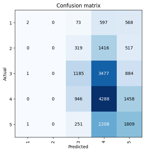

The model is now predicting 5s. Although now it’s not predicting any 1s or 2s! I’ll see if there’s a better learning rate for this architecture:

model = DotProductBiasCE(n_users, n_movies, n_factors=50)
learn = Learner(dls, model, loss_func=CrossEntropyLossFlat(), metrics=accuracy)

learn.lr_find()

SuggestedLRs(valley=0.005248074419796467)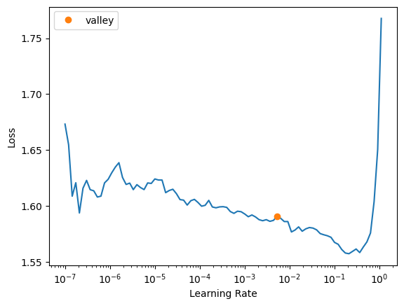

I’ll try a learning rate of 0.1, which is two orders of magnitude larger than 5e-3.

model = DotProductBiasCE(n_users, n_movies, n_factors=50)
learn = Learner(dls, model, loss_func=CrossEntropyLossFlat(), metrics=accuracy)

learn.fit_one_cycle(5, 0.1, wd=0.1)

epoch	train_loss	valid_loss	accuracy	time
0	1.402151	1.460189	0.337900	00:14
1	1.410952	1.438032	0.348000	00:13
2	1.353970	1.407190	0.370100	00:13
3	1.232812	1.351564	0.401050	00:13
4	1.070482	1.324203	0.415400	00:14

The higher learning rate improved the accuracy by about 5%. Looking at the confusion matrix, here are some observations—the model is predicting 1s and 2s better than before and the rating of 4 is still the best predicted rating (62% of all actual 4s are predicted as 4s). However, the model is still predominantly predicting 3s and 4s.

interp = ClassificationInterpretation.from_learner(learn)
interp.plot_confusion_matrix()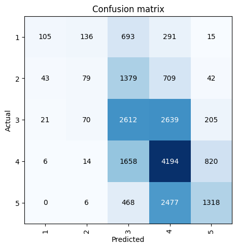

I’ll also check that fastai is automatically applying softmax so that the final activations add up to 1.00:

probs, _ = learn.get_preds(dl=dls.valid)
probs.sum(dim=1)

tensor([1.0000, 1.0000, 1.0000,  ..., 1.0000, 1.0000, 1.0000])

probs.sum(dim=1).sum() # should equal 20k

tensor(20000.)

Final Thoughts

I’ll recap this exercise by displaying the visual comparison between DotProductBias and the final DotProductBiasCE (without y_range and sigmoid_range).

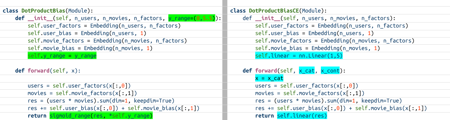
Visual inspection of DotProductBias Modules

My main takeaway from this exercise is that what may work for one architecture may not necessarily work for another. In this example when passing the dot product through the sigmoid function before passing it through a linear layer, the model did not predict any 5s even though there were many actual 5 ratings in the dataset.

Another takeaway is that I wasn’t able to compare two models that used different metrics (RMSE vs. accuracy). So I’m limited in my ability to say which model performed “better”. I asked Claude for ideas on how to compare these two models and it came up with the following:

• Convert RMSE to accuracy
  • Round continuous predictions to nearest integer
  • Calculate accuracy using rounded predictions
  • Compare this accuracy to the categorical model
• Convert accuracy to RMSE-like metric:
  • Calculate average error for categorical predictions
  • Compare this to the continuous model’s RMSE
• Use normalized metrics:
  • Normalize RMSE: RMSE / (max_rating - min_rating)
  • Normalize accuracy: (accuracy - random_guess_accuracy) / (1 - random_guess_accuracy)
  • Compare normalized values

I’ll poke around online (I’ve also asked about this on Twitter and the fastai forums) to see if there are thoughts on or examples of such comparisons, and then follow up with some exploration in a future blog post.

I hope you enjoyed this exercise! Follow me on Twitter @vishal_learner.