How Does Stable Diffusion Work?
Background
In this blog post, I’ll review the concepts introduced in the second half of the Lesson 9 video from the fastai course (Part 2: Deep Learning Foundations to Stable Diffusion). Note that I will not be covering any of the math of Stable Diffusion in this blog post. As Jeremy says in the video:
the way Stable Diffusion is normally explained is focused very much on a particular mathematical derivation. We’ve been developing a totally new way of thinking about Stable Diffusion and I’m going to be teaching you that. It’s mathematically equivalent [to other approaches] but it’s actually conceptually much simpler [and it can take you in really innovative directions].
I’ll start with the main takeaway from this lesson, which is this table that shows the three types of models involved in stable diffusion, the inputs they take and the outputs they produce:
| Model | Inputs | Outputs |
|---|---|---|
| U-Net | Somewhat Noisy Latents | Noise |
| VAE’s Decoder | Small Latents Tensor | Large Image |
| CLIP Text Encoder | Text | Embedding |
The noise predicted by the U-Net (which receives as input somewhat noisy latents, text embeddings generated by the CLIP Text Encoder and a time step) is (iteratively) scaled and subtracted from the somewhat noisy latents to create denoised latents which are input to the VAE’s Decoder, which reconstructs from them larger images.
The Magic API
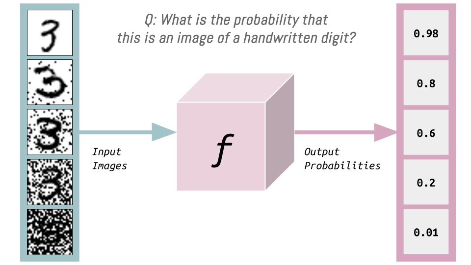
We start by considering some blackbox web API (some “magic API”) that takes as inputs images of handwritten digits and outputs the probability that the inputs are handwritten digits. In other words, this magic API answers the question: what’s the probability that this is an image of a handwritten digit?
Let’s consider this API to be some function \(f\).
Varying the Inputs fo \(f\)
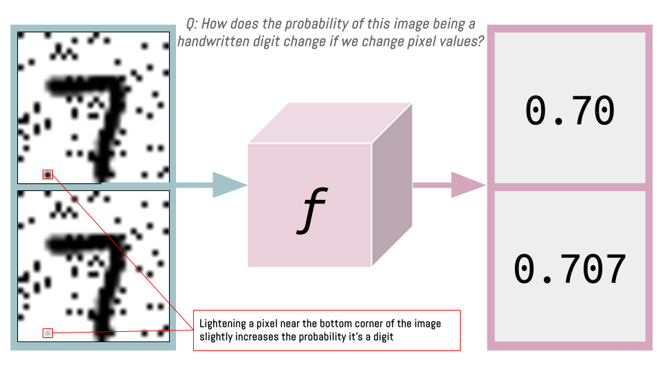
In the case of MNIST we have 28x28 = 784 pixels (or variables) in our input. Changing the value of each of these pixels will change the probability of it being a handwritten digit.
For example, digits usually don’t have dark pixels near the bottom corners. If we lighten such a pixel (highlighted in red below) and pass it through the function \(f\), the probability of it being a handwritten digit will slightly improve (e.g. from 0.7 to 0.707).
We can do this for each pixel: determine whether making it lighter or darker makes it more like a handwritten digit.
The Gradient of the Loss With Respect to the Pixels
There exists a loss function that is a function of the weights of a neural net (in our case, our “magic API” or function \(f\)) and the pixel values \(X\):
\[\text{loss} = g(w,X)\]
This loss function could be the MSE (Mean Squared Error) between our targets and predictions but for now just assume it’s some function \(g\).
What happens to the loss as we change \(X\)? Our \(X\) consists of 28x28=784 pixels, and our loss function can change with respect to each one of those pixels (also known as partial derivatives):
\[\frac{\partial{\text{loss}}}{\partial{X_{(1,1)}}}, \frac{\partial{\text{loss}}}{\partial{X_{(1,2)}}}, \frac{\partial{\text{loss}}}{\partial{X_{(1,3)}}}, ..., \frac{\partial{\text{loss}}}{\partial{X_{(28,28)}}}\]
We can rewrite this compactly as:
\[\nabla_X \text{loss}\]
Which we read as: the gradient of the loss with respect to \(X\).
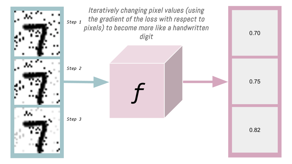
We can change the pixel values according to this gradient to get our image looking closer to a handwritten digit. In practice, we subtract the gradient (multiplied by some constant \(c\)) from the image pixel data, and do this iteratively (as illustrated below), calculating a new gradient each time:
If we have access to our magic function \(f\), we can generate images that look like handwritten digits. And assuming that magic API is using python, we don’t even need access to \(f\), we just need access to f.backward and X.grad.
Creating the Magic Function \(f\) (the U-Net)
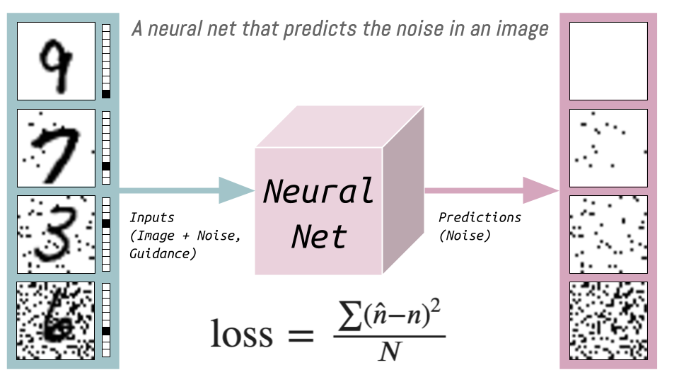
Generally, in this course, when there’s some magic blackbox that we want to exist and it doesn’t exist, we create a Neural Net and we train it. We want to train a Neural Net that tells us which pixels to change to a make an image look more like a handwritten digit.
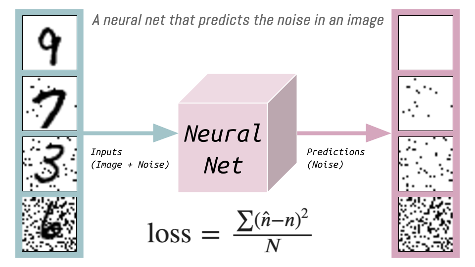
The training data (noisy images of digits) and targets (the amount of noise added) for this Neural Net I’ve illustrated as the following:
The loss function is the MSE between the predicted noise \(\hat{n}\) and actual noise \({n}\) (\(N\) is the number of images) which is used then to update the weights of the neural net.
How much do we have the change an image (noisy digit) by to make it more digit-like? We have to subtract the noise!
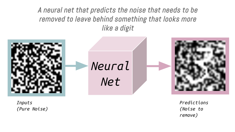
We end up with a neural net that can take as an input pure noise and predict the amount of noise that needs to be removed so that what is left behind looks the most like a handwritten digit. To illustrate:
This process of predicting and subtracting the noise (multiplied by a constant) that needs to be removed occurs multiple times, each time getting closer to leaving behind the pixels for a digit.
The neural net that we use for this is the U-Net.
When You Don’t Have a Room Full of TPUs: The Autoencoder
In practice, we want to generate more than just 28x28=784 pixels of handwritten digits. We want to generate 512x512x3=786432 pixels of full color, high resolution images. Training a model on millions of these images will take a lot of time and compute. How do we do this more efficiently?
We already know that lossy compression can take place with images, like JPEGs, where the size of the image file (in bytes) is much smaller than the bytes of actual pixels (height pixels x width pixels x number of channels).
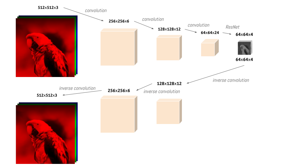
We can compress large images into small latents using a neural network (with convolutions and ResNet blocks), and then reconstruct the images from these small latents (using inverse convolutions):
This neural net compresses 786,432 pixels into 16,384 pixels, a 48x compression!
During training, we input 512x512x3 images and the neural net will initially output 512x512x3 random noise (as the weights are randomly instantiated). The loss function is the MSE between the input images and the output images. As the loss decreases, the output images look closer to the inputs. This model, something that gives back what you give it, is called an autoencoder.
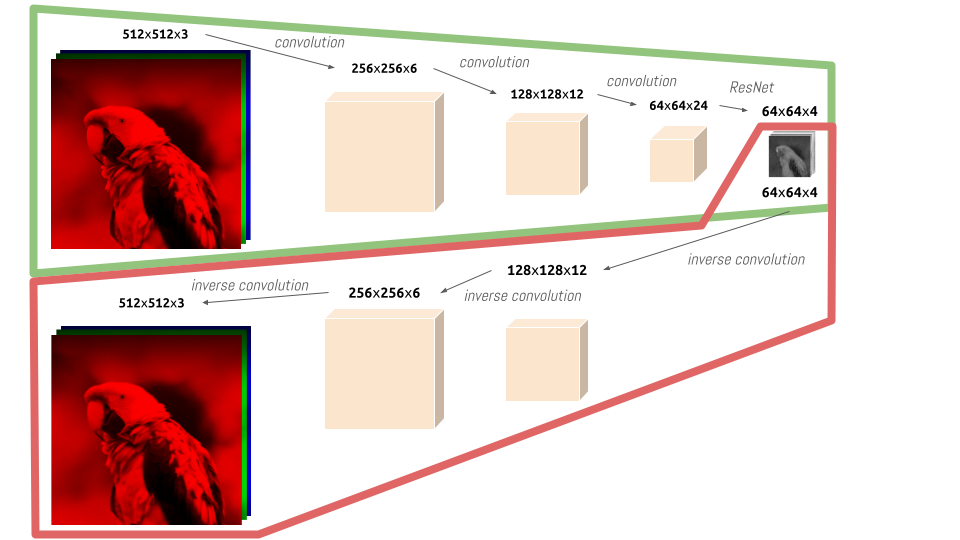
The beauty of this model is when you split it in “half” into an encoder (green) and a decoder (red):
We can feed full-size images to the encoder and it will output latents that are used as inputs to the U-Net (for training and inference).
The final denoised latents (from U-Net) become the inputs to the decoder which outputs full-size images.
In this way we can train the U-Net on 48x less data because we are able to recover most of the information with our trained autoencoder’s decoder!
The autoencoder that we will use is called a VAE (Variational Autoencoder).
The use of latents is entirely optional:
generally speaking, we would rather not use more compute than necessary, so, unless you’re trying to sell the world a room full of TPUs, you would probably rather everybody was doing stuff in the thing that’s 48 times smaller. So the VAE is optional but it saves us a whole lot of time and a whole lot of money. So that’s good.
Encoding “A cute teddy”: CLIP (Contrastive Language-Image Pre-Training)
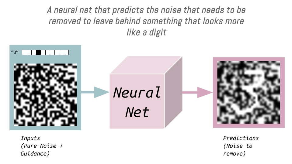
How could we modify our pipeline so that we could tell the U-Net that we wanted it to give us the noise to remove and leave behind not just any digit, but a particular digit, like 3?
We want to pass into the model (as input) “3” as a one-hot encoded vector so it predicts the noise we need to remove (to leave behind a “3”). There are 10 elements in this vector representing each possible digit in the MNIST dataset, 0-9:
During training, in addition to passing in noisy digits, we pass in a one-hot encoded representation of that digit. The model thus learns what noise needs to be removed to leave a particular digit behind:
That’s a straightforward way to give it guidance. When the guidance gets more complex than single digits, one-hot encoding no longer works:
we can’t create every possible sentence that’s been uttered in the whole world and then create a one-hot encoded version of every sentence in the world
The solution? Embeddings!!
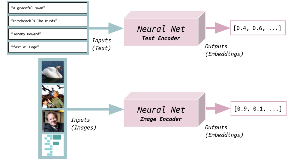
We can train two neural nets: one that takes in as inputs texts and outputs embeddings (vectors w/ numbers) and one that takes in as inputs images and also outputs embeddings.
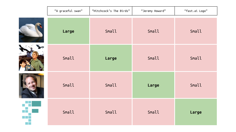
For each pair of text and image, we want the model to output text embeddings that are similar to the corresponding image’s embeddings:
To achieve this, we use something called contrastive loss (the “CL” in “CLIP”). Optimizing this loss means increasing the dot product between related image/text pairs (e.g. “a graceful swan” and the image of the swan) and decreasing the dot product between unrelated image/text pairs (e.g. “a graceful swan” and the fast.ai logo).
The result is a model where similar texts:
- “a graceful swan”
- “a beautiful swan”
- “such a lovely swan”
will produce similar embeddings as they correspond to similar images.
These two models put text and images into the same space; they are a multimodal set of models.
We can now embed “a cute teddy” and pass it to a U-Net (that is trained on input images and corresponding text embeddings) and it will return the noise that needs to be removed from the somewhat noisy latent to leave behind something that looks like a cute teddy.
Weird and Confusing “Time Steps”: The Inference Process
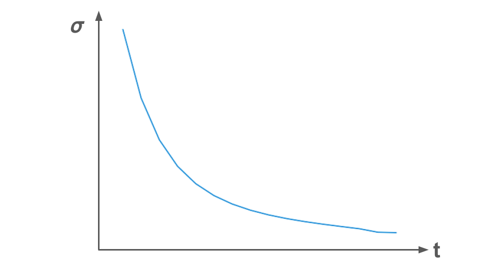
When we’re training the U-Net, we pick a random amount of noise to add to each input image (or latent). One way to pick it is to select a certain “time step” (an overhang from the mathematical formulation of diffusion) for which there is a corresponding amount of noise. A “noising schedule” will look something like this:
You may also see the standard deviation of the noise being used referred to as the Greek letter beta (\(\beta\)).
At inference time (generating a picture from pure noise) the model will create some hideous and random thing:
We multiply the predicted noise by a constant (a la learning rate, but for updating pixels, not weights) and subtract it from the pixels. We have to take these incremental steps toward fully denoising the image because our model didn’t train on the hideous image above, so it doesn’t know how to go in one step (at the time of this video) from hideous-random-thing to a high resolution image of something plausible.
The diffusion sampler is used to decide how much noise to add during training and how much noise to subtract during inference.
If you squint—diffusion samplers look like optimizers. We have tricks we can use (like momentum, or adaptive learning rate) for optimizers and fastai early research at the time showed that we can use similar ideas for diffusion.
U-Nets traditionally also take as input the time step t. If a model is trained knowing how much noise is used, the better it will be at removing noise.
Jeremy thinks this premise is incorrect, because neural nets can very easily predict how noisy something is.
If you step passing the U-Net the time step t:
things stop looking like differential equations and they start looking more like optimizers. Early results suggest that when we re-think the whole thing as being about learning rates and optimizers, maybe it actually works better.
If we stop centering the concepts that are related to the mathematical formulation of diffusion, such as using the mathematically easy Mean Squared Error as loss, we can use something more sophisticated like perceptual loss to evaluate if our outputs resemble our targets (e.g. handwritten digits).
Final Thoughts
I’ll finish this blog post by reiterating what Jeremy emphasized is the main takeaway from this lesson: understanding what the inputs and outputs are of the different models used for diffusion:
| Model | Inputs | Outputs |
|---|---|---|
| U-Net | Somewhat Noisy Latents | Noise |
| VAE’s Decoder | Small Latents Tensor | Large Image |
| CLIP Text Encoder | Text | Embedding |
I hope you enjoyed this blog post! Follow me on Twitter @vishal_learner.
