Comparing ~100k Random Numbers Generated with Different Methods

python

machine learning

deep learning

In this blog post, I generate close to 100k random numbers using 5 different methods: ANU Quantum numbers, Python’s random module, NumPy, PyTorch and a custom implementation from Lesson 10 of the fastai course (Part 2). I am surprised by the results!

Author

Vishal Bakshi

Published

September 3, 2024

Background

In this notebook I’ll run some experiments to compare random numbers generated with the following approaches:

The Australian National University Quantum Numbers API
random (Python Standard Library)
numpy.random.randint
torch.randint
The rand function from Lesson 10 of the fastai course (Part 2)

Getting ~100k Random Numbers from the ANU API

I refactored code from the ANU documentation into the following function:

import json, requests, random
import pandas as pd
import matplotlib.pyplot as plt
import numpy as np
import torch
from scipy import stats

def get_anu(qrn_key, dtype, length, blocksize=1):
  QRN_URL = "https://api.quantumnumbers.anu.edu.au/"
  params = {"length": length, "type": dtype, "size": blocksize}
  headers = {"x-api-key": qrn_key}

  response = requests.get(QRN_URL, headers=headers, params=params)

  if response.status_code == 200:
    js = response.json()
    if js["success"] == True:
        print(js["data"])
    else:
        print(js["message"])
  else:
    print(f"Got an unexpected status-code: {response.status_code}")
    print(response.text)

So that I could run through a loop for multiple API calls. I ended up using 3 calls for testing so only generated 99328 total random numbers (1024 per 97 API calls).

results = []

for i in range(100):
  res = get_anu(qrn_key=QRN_KEY, dtype="uint8", length=1024, blocksize=1)
  results.extend(res)

len(results)

I have uploaded the list of random numbers to this gist. You can use the following helper function to load the txt file into a python list:

# Loading the list from a file
def load_list(file_name):
    with open(file_name, 'r') as file:
        return json.load(file)
        
# Load the list
results = load_list("anu_random_numbers.txt")

Viewing the Random Numbers

Let’s take a moment and appreciate the beauty of truly random numbers! It looks like static on an old TV screen:

results = pd.Series(results)
plt.scatter(results.index, results.values, s=1, alpha=0.3);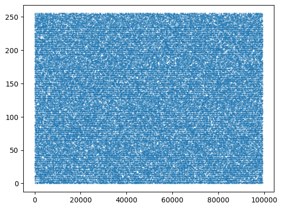

Generating Random Numbers Using Other Approaches

I’ll now generate 99,328 random numbers using the following methods:

random (Python Standard Library)
numpy.random.randint
torch.randint
The rand function from Lesson 10 of the fastai course (Part 2)

Note that the ANU random numbers are between 0-255.

the data type must be 'uint8' (returns integers between 0-255)

results.min(), results.max()

(0, 255)

`random` (Python Standard Library)

From the Python docs:

random.randint(a, b)

Return a random integer N such that a <= N <= b. Alias for randrange(a, b+1).

random.randint(0,255)

py_results = pd.Series([random.randint(0,255) for _ in range(99328)])
py_results.min(), py_results.max()

(0, 255)

Visibly, there’s not much difference between this scatter plot and the ANU random numbers.

plt.scatter(py_results.index, py_results.values, s=1, alpha=0.3);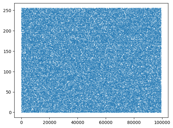

`numpy.random.randint`

The NumPy functionality is a bit different, it excludes the upper bound that you provide:

Return random integers from low (inclusive) to high (exclusive).

np.random.randint(0, 256)

np_results = pd.Series([np.random.randint(0, 256) for _ in range(99328)])
np_results.min(), np_results.max()

(0, 255)

plt.scatter(np_results.index, np_results.values, s=1, alpha=0.3);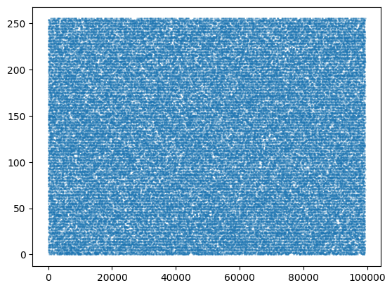

`torch.randint`

PyTorch does it similar to NumPy:

Returns a tensor filled with random integers generated uniformly between low (inclusive) and high (exclusive).

But also asks the shape of the tensor you want as a parameter.

pt_results = pd.Series(torch.randint(0, 256, (99328,)))
pt_results.shape, pt_results.min(), pt_results.max()

((99328,), 0, 255)

plt.scatter(pt_results.index, pt_results.values, s=1, alpha=0.3);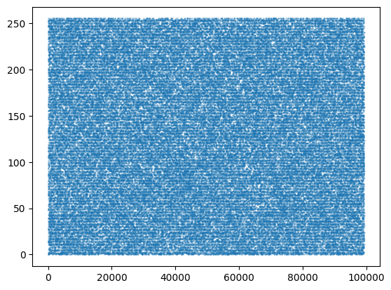

Custom `rand` Implementation

In Lesson 10 of the fastai course (Part 2), Jeremy implements the following from-scratch random number generator:

rnd_state = None
def seed(a):
    global rnd_state
    a, x = divmod(a, 30268)
    a, y = divmod(a, 30306)
    a, z = divmod(a, 30322)
    rnd_state = int(x)+1, int(y)+1, int(z)+1

seed(457428938475)
rnd_state

(4976, 20238, 499)

def rand():
    global rnd_state
    x, y, z = rnd_state
    x = (171 * x) % 30269
    y = (172 * y) % 30307
    z = (170 * z) % 30323
    rnd_state = x,y,z
    return (x/30269 + y/30307 + z/30323) % 1.0

rand()

0.7645251082582081

Since this implementation generates floats between 0 and 1, I’ll have to handle it a bit differently:

rand_results = pd.Series([int(rand()*256) for _ in range(99328)])
rand_results.min(), rand_results.max()

(0, 255)

plt.scatter(rand_results.index, rand_results.values, s=1, alpha=0.3);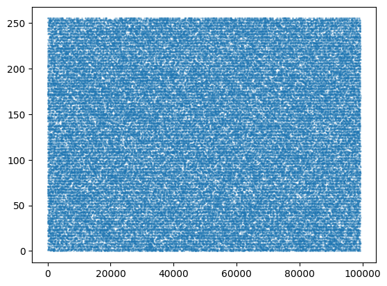

Comparing Random Numbers Generated with Different Methods

Upon visual inspection, the distributions of 99328 random numbers generated by the different methods look similar.

With the help of Claude, I’ll apply a few statistical tests and compare the results across all five sets of (differently generated) random integers:

def random_analysis(data_sets, names):
    results = []

    # Create a 2x3 grid of subplots
    fig, axs = plt.subplots(2, 3, figsize=(10, 5))
    axs = axs.flatten()

    for i, (data, name) in enumerate(zip(data_sets, names)):
        # Basic statistical measures
        mean = np.mean(data)
        variance = np.var(data)
        std_dev = np.std(data)

        # Chi-square test for uniformity
        observed_freq, _ = np.histogram(data, bins=256, range=(0, 255))
        expected_freq = len(data) / 256  # Assuming uniform distribution
        chi2_stat, chi2_p = stats.chisquare(observed_freq, f_exp=[expected_freq]*256)

        # Kolmogorov-Smirnov test
        ks_stat, ks_p = stats.kstest(data, 'uniform', args=(0, 256))

        results.append({
            'Name': name,
            'Mean': mean,
            'Variance': variance,
            'Std Dev': std_dev,
            'Chi-square Statistic': chi2_stat,
            'Chi-square p-value': chi2_p,
            'KS Statistic': ks_stat,
            'KS p-value': ks_p
        })

        # Plot histogram in the corresponding subplot
        axs[i].hist(data, bins=256, range=(0, 255), density=True)
        axs[i].set_title(f'Histogram for {name}')
        axs[i].set_xlabel('Value')
        axs[i].set_ylabel('Frequency')

    # Remove any unused subplots
    for j in range(i+1, len(axs)):
        fig.delaxes(axs[j])

    plt.tight_layout()
    plt.show()

    return pd.DataFrame(results)

Again, by visual inspection, the histograms of the differently generated random integers look similar, if not the same. It’s interesting to note that there are dips in the distribution where certain integers have significantly lower occurences than others.

data_sets = [results, py_results, np_results, pt_results, rand_results]
names = ['Quantum', 'Python Random', 'NumPy Random', 'Torch Random', 'Custom Random']

res = random_analysis(data_sets, names)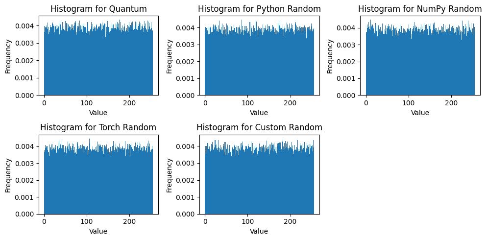

Next, I’ll interpret the various statistics calculated.

For a uniform distribution (between \(a=0\) and \(b=255\)), the expected value for the mean, variance and standard deviation are as follows:

\[\text{Mean: } \mu = \frac{a + b}{2} = \frac{0 + 255}{2} = 127.5\]

\[\text{Var: } \sigma^2 = \frac{(b - a + 1)^2 - 1}{12} = \frac{(255 - 0 + 1)^2 - 1}{12} = \frac{256^2 - 1}{12} \approx 5461.25\]

\[\text{Std: } \sigma = \sqrt{5461.25} \approx 73.91\]

The method with the mean closest to the expected value is numpy.random.randint (127.502). The closest variance to the expected value is the ANU Quantum method (5459.429).The closes standard deviation is also the ANU Quantum method (73.888).

res

	Name	Mean	Variance	Std Dev	Chi-square Statistic	Chi-square p-value	KS Statistic	KS p-value
0	Quantum	127.584518	5459.429128	73.887950	216.123711	0.963092	0.004792	0.020812
1	Python Random	127.677402	5451.449199	73.833930	246.185567	0.642552	0.004651	0.027113
2	NumPy Random	127.502638	5482.749449	74.045590	277.453608	0.159672	0.006041	0.001416
3	Torch Random	127.531039	5477.553241	74.010494	237.572165	0.776473	0.005477	0.005147
4	Custom Random	127.894380	5469.084638	73.953260	289.896907	0.065635	0.004671	0.026121

Next, I’ll look at the chi-square statistic, where lower values are better. The Quantum method has the lowest chi-square statistic with the highest p-value, meaning it’s the closest to a uniform distribution.

Next, looking at the KS statistic, from the SciPy docs, it measures:

the distance between the empirical distribution function and the hypothesized cumulative distribution function

Again, lower values are better. However, the p-values are all lower than 0.05, indicating that the null hypothesis (that the data comes from a uniform distribution) should be rejected. Claude provided the following insight:

The KS test is very sensitive, especially with large sample sizes. With 99,328 numbers, even small deviations from perfect uniformity can lead to statistically significant results.

My interpretation of this is that it’s not a perfectly uniform distribution.

Reducing the Number of Samples

I’ll run these tests with a much lower number of samples and see if that changes any of the statistics significantly.

data_sets = [results[:10000], py_results[:10000], np_results[:10000], pt_results[:10000], rand_results[:10000]]
names = ['Quantum', 'Python Random', 'NumPy Random', 'Torch Random', 'Custom Random']

res = random_analysis(data_sets, names)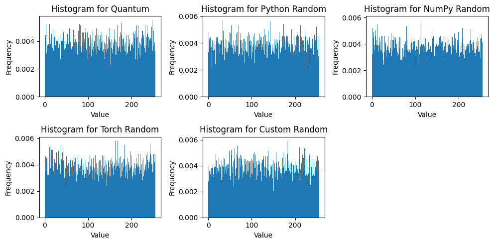

Using only 10,000 samples each, the statistics have changed:

The Quantum method no longer has the variance closest to the expected value of 5461.25. That claim belongs to Python’s random module (which has the closest value, 73.9 to the expected standard deviation of 73.91).
NumPy again has the closet mean to the expected value of 127.5.
The Chi-square statistics have changed, with Python leading the way (although all of the methods still have a high p-value).
The KS statistic has also significantly changed: all methods now have a p-value greater than 0.05, indicating that the null hypothesis (that they belong to a uniform distribution) cannot be rejected.

res

	Name	Mean	Variance	Std Dev	Chi-square Statistic	Chi-square p-value	KS Statistic	KS p-value
0	Quantum	127.6421	5556.331208	74.540802	236.6720	0.788774	0.008306	0.492614
1	Python Random	128.3820	5461.679276	73.903175	234.7264	0.814062	0.007994	0.542459
2	NumPy Random	127.5575	5459.439094	73.888017	236.2112	0.794925	0.009550	0.319373
3	Torch Random	127.9056	5668.028889	75.286313	265.1392	0.318255	0.015931	0.012354
4	Custom Random	127.8054	5392.456331	73.433346	276.6592	0.167893	0.008838	0.413184

Final Thoughts

I was surprised that the random numbers generated by alternative approaches to the ANU Quantum generated were comparable to it! I was also surprised that even the Quantum-generated random numbers were not perfect—they still deviated from the expected values of a uniform distribution. I was also not expecting the statistics to change so dramatically depending on the number of samples analyzed.

This is my first true foray into the world of random number generation (outside of setting seeds during training) and I have probably only scratched the surface. I look forward to being more mindful about random numbers in the future.

Thanks for reading this blog post! Follow me on Twitter @vishal_learner.