Initial Experiments with Imagenette

python

fastai

deep learning

tinyscalelab

This post walks through initial 5 epoch experiments on the small Imagenette dataset as I try to get onto the leaderboard.

Author

Vishal Bakshi

Published

June 1, 2025

from fastai.vision.all import *
from fastai.callback.wandb import WandbCallback
import wandb
import pandas as pd
import matplotlib.pyplot as plt

Background

In this blog post I’m going to share my initial experiments as I try to get on the imagenette leaderboard.

Imagenette is a subset of 10 easily classified classes from Imagenet (tench, English springer, cassette player, chain saw, church, French horn, garbage truck, gas pump, golf ball, parachute).

This exercise is a bit of a detour but related to my TinyScaleLab project in which I’m trying to analyze the relationship between downstream capabilities and training dynamics for tiny language models (5M-125M) trained on the TinyStories dataset.

I was running some initial rough 1 epoch training runs with my 5M architecture to find the best batch size for training efficiency (memory usage and training speed). I encountered a peculiar result which was counterintuitive to me:

Metric	bs=64	256	1024	2048	4096
Time	3hr	1hr	0.5hr	0.5hr	OOM
Train loss	3.58	3.46	4.42	5.57	OOM
Eval loss	3.58	3.46	4.43	5.57	OOM

I was expecting that increase the batch size would:

speed up training
decrease loss

However, increasing batch size from 1024 to 2048 did not speed up training, and increasing batch size from 256 to 2048 did not improve the loss. As always, when I run into something unexpected, I post it on Twitter. I received a number of insightful comments:

We covered this in some of our earlier courses - lower batch sizes provide more updates, which should give better results for a fixed # epochs.
— Jeremy Howard (@jeremyphoward) May 27, 2025

The batch size of 256 was certainly providing more updates in one epoch than a batch size of 1024 or 2048. It’s interesting to note that a batch size of 64, even though providing 4x the number of updates as 256, had a higher loss at the end of the epoch. It’s important to note that I did not measure downstream performance for this experiment.

TinyStories is a pretty homogeneous dataset, so one doesn't need as large of a batch size to achieve a smooth gradient compared to a more diverse pretraining dataset.

You'll want to set the batch size balancing speed and performance.
— Benjamin Warner (@benjamin_warner) May 27, 2025

This was another interesting point. The benefit of increasing batch size is to get a closer representation to the overall dataset. Since the TinyStories dataset is quite homogenous (all dataset items are children’s stories) a smaller batch size will be sufficiently representative of the full dataset. On the flip side, if we have a dataset like the PETS dataset, and used a small batch size of say 32, we could imagine a scenario where the batch only includes images of a single class. The model, which has been learning about a diverse set of animals to this point will perform poorly and the loss will spike. Larger models, having more parameters, may not recover from this spike like small models can. Furthermore, if the dataset contains mislabeled images and you are unfortunate to get a batch of incorrectly labeled cats, your loss spike will be combined with the model learning incorrect information. These were points discussed in a fastai study group!

Also, one heuristic that people use is that in most scenarios, you can scale the lr proportionally to the bs.

Larger bs, better but less frequent updates, can take longer steps.

Smaller bs, more frequent updates, but need to take smaller steps due to worse direction of updates.
— Radek Osmulski 🇺🇦 (@radekosmulski) May 27, 2025

In my case, I had used the same learning rate for all batch sizes, and did not utilize the benefit of larger batch sizes taking longer steps (higher learning rate).

Jeremy also encouraged me to do some imagenette speedruns, which is why we’re here!

You should maybe try doing some imagenette speed-running – it's a good way to get an intuitive understanding of these issues.
— Jeremy Howard (@jeremyphoward) May 27, 2025

Approach and Results

My data prep and training code can be viewed in the “appendix” below. Before I did this exercise, I ran the code in the fastai “Training Imagenette” tutorial which is where most of the code below comes from. I’ll share my approach and results in this section. I wanted to break this exercise (of trying to get onto the Imagenette leaderboard) into smaller steps, so I focused this notebook on training with a batch size of 64, for three learning rates (1e-4, 1e-3 and 1e-2) for three models: xse_resnext50 (25.6M), xresnet34 (21.3M), xresnet18 (11.2M).

Accuracy Curves

Since I’m most interested in competing on the leaderboard, I’ll focus on observing the accuracy curves of these models, all trained on 5 epochs of the same training/validation split.

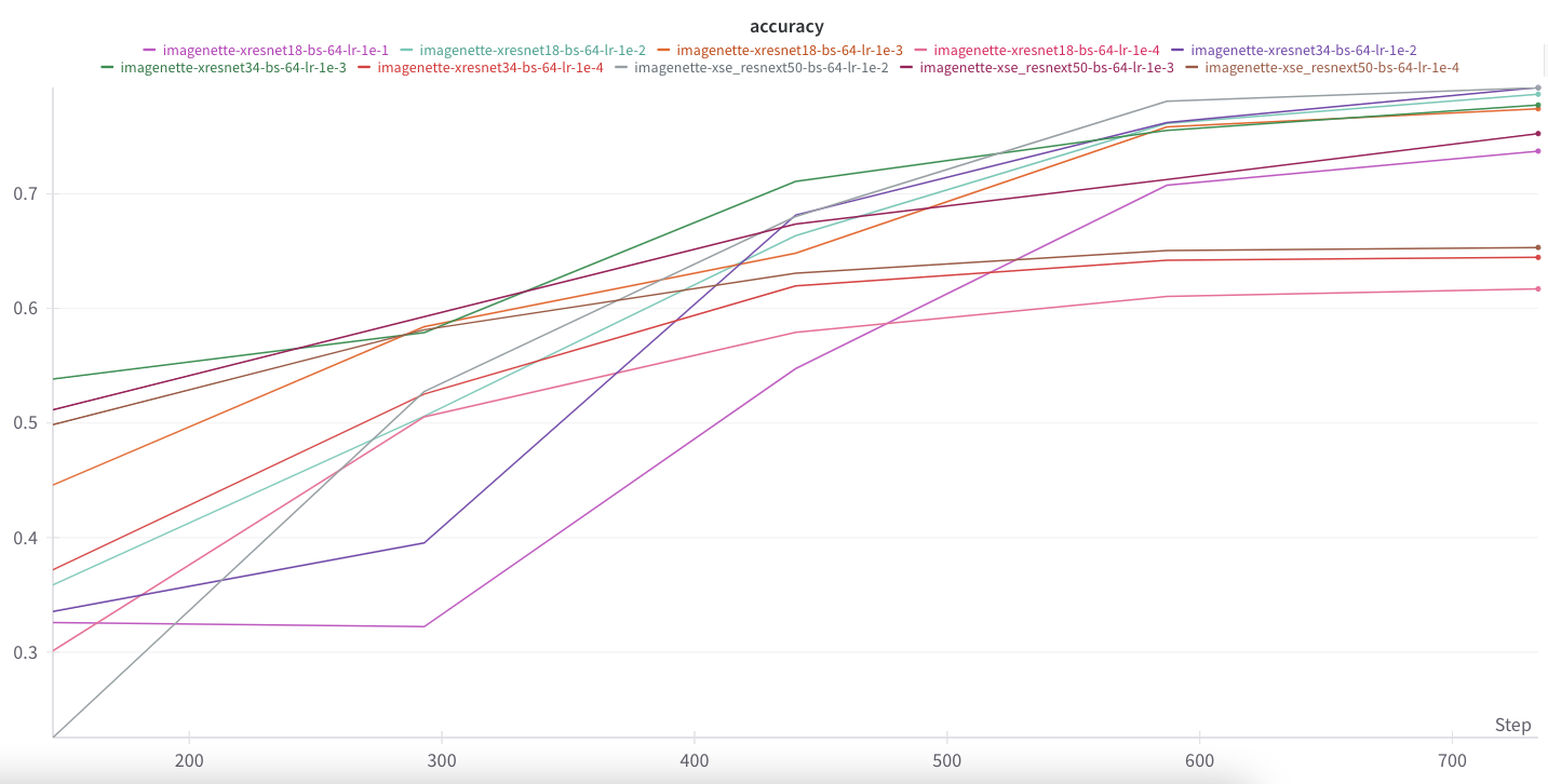
The models/learning rate combination with the highest accuracy is xresnet34/1e-2 and xse_resnext50/1e-2. xresnet18/1e-2 is surprisingly competitive at half the parameter count. There is a clear hierarchy of learning rates, 1e-2 performs the best for all three models, followed by 1e-3 and then 1e-4. I used lr_find for each model and found that xresnet18 was stable for 1e-1 though it performs second-to-last place in accuracy for that model.

Model/Learning Rate	Accuracy
xresnet34/1e-2	0.7929
xse_resnext50/1e-2	0.7926
xresnet18/1e-2	0.7870
xresnet34/1e-3	0.7776
xresnet18/1e-3	0.7743
xse_resnext50/1e-3	0.7526
xresnet18/1e-1	0.7373
xse_resnext50/1e-4	0.6532
xresnet34/1e-4	0.6446
xresnet18/1e-4	0.6171

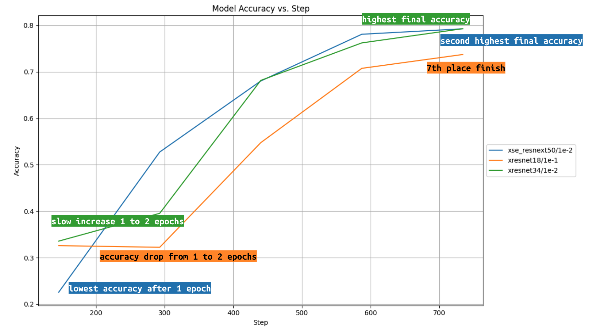
Other notable observations:

xse_resnext50/1e-2 starts out with the lowest accuracy, but then quickly catches up and finally beats out all other models/LRs but one.
xresnet18/1e-1 accuracy decreases from epoch 1 to 2, then catches up to finish in 7th place.
xresnet34/1e-2 accuracy increasing at slower rate from epoch 1 to 2 than from epoch 2 to 3, catching up quickly to finish in the top spot.

Next Steps

I want to focus on a couple of thoughts Jeremy shared:

Maybe on the way you'll want to create some tables like you're making there, but I rarely find them as interesting as small targeted iterations changing one thing at a time.
— Jeremy Howard (@jeremyphoward) May 27, 2025

Last year I worked through Jeremy’s Kaggle Paddy Docter competition live coding series and learned a ton about just that—small targeted iterations changing one thing at a time.

I’m not quite sure what my plan will be for this Imagenette leaderboard exercise, but I since I started this exploration with the intent to build intuition about batch size/learning rate and downstream performance, it makes sense to pick my best 2-3 models and vary the batch size and learning rate next.

I also am keen on working with Benjamin Warner’s fastxtend (which I used last year in the BirdCLEF24 Kaggle competition to finish in the top 34%) and optimi libraries. I’m particularly keen on trying out the different data augmentation techniques provided in fastxtend when I train for longer than 5 epochs.

I’m trying to grow my YouTube channel, so if you like my content, please subscribe!

Appendix

Data Prep

path = untar_data(URLs.IMAGENETTE_160)

100.01% [99008512/99003388 00:03<00:00]

lbl_dict = dict(
    n01440764='tench',
    n02102040='English springer',
    n02979186='cassette player',
    n03000684='chain saw',
    n03028079='church',
    n03394916='French horn',
    n03417042='garbage truck',
    n03425413='gas pump',
    n03445777='golf ball',
    n03888257='parachute'
)

imagenette = DataBlock(blocks = (ImageBlock, CategoryBlock),
                       get_items = get_image_files,
                       get_y = Pipeline([parent_label, lbl_dict.__getitem__]),
                       splitter = GrandparentSplitter(valid_name='val'),
                       item_tfms = RandomResizedCrop(128, min_scale=0.35),
                       batch_tfms = Normalize.from_stats(*imagenet_stats))

dls = imagenette.dataloaders(path, bs=64)
dls.show_batch()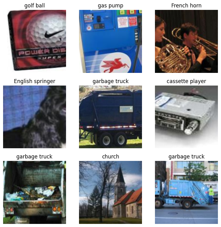

Training Code

I chose to run everything on a Colab Pro A100 GPU to maximize speed.

xse_resnext50

learn = vision_learner(dls, xse_resnext50, metrics=accuracy, pretrained=False)
learn.lr_find()

SuggestedLRs(valley=0.0004786300996784121)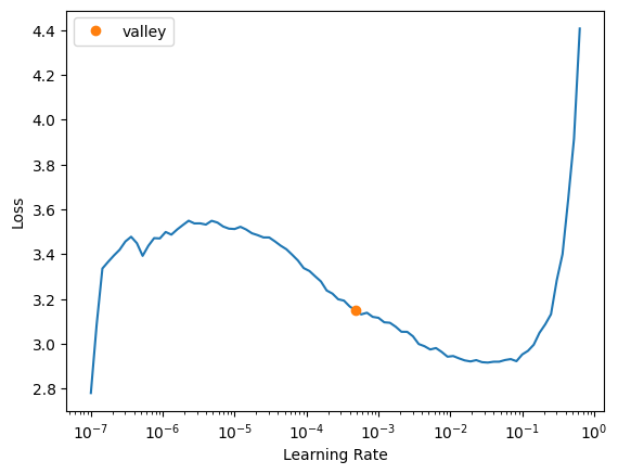

wandb.login()

True

wandb.init(
    project="tinyscale-lab",
    name="imagenette-xse_resnext50-bs-64-lr-1e-4",
)

learn = vision_learner(dls, xse_resnext50, metrics=accuracy, pretrained=False, cbs=WandbCallback())
learn.fit_one_cycle(5, 1e-4)

epoch	train_loss	valid_loss	accuracy	time
0	2.437292	1.562259	0.498599	00:15
1	1.898073	1.330338	0.581401	00:15
2	1.625788	1.184957	0.630828	00:15
3	1.491183	1.138762	0.650446	00:15
4	1.425214	1.119943	0.653248	00:15

wandb.finish()

wandb.init(
    project="tinyscale-lab",
    name="imagenette-xse_resnext50-bs-64-lr-1e-3",
)

learn = vision_learner(dls, xse_resnext50, metrics=accuracy, pretrained=False, cbs=WandbCallback())
learn.fit_one_cycle(5, 1e-3)

epoch	train_loss	valid_loss	accuracy	time
0	2.115490	1.610692	0.511592	00:15
1	1.563322	1.359540	0.592866	00:15
2	1.205948	1.041064	0.673631	00:15
3	0.988717	0.896793	0.712611	00:15
4	0.865071	0.776657	0.752611	00:15

wandb.finish()

wandb.init(
    project="tinyscale-lab",
    name="imagenette-xse_resnext50-bs-64-lr-1e-2",
)

learn = vision_learner(dls, xse_resnext50, metrics=accuracy, pretrained=False, cbs=WandbCallback())
learn.fit_one_cycle(5, 1e-2)

epoch	train_loss	valid_loss	accuracy	time
0	2.025805	4.565277	0.225478	00:15
1	1.586654	1.567472	0.527389	00:15
2	1.162438	0.994889	0.680255	00:15
3	0.868640	0.672154	0.780892	00:15
4	0.703673	0.635068	0.792611	00:15

wandb.finish()

xresnet34

learn = Learner(dls, xresnet34(n_out=10), metrics=accuracy)
learn.lr_find()

SuggestedLRs(valley=0.0005754399462603033)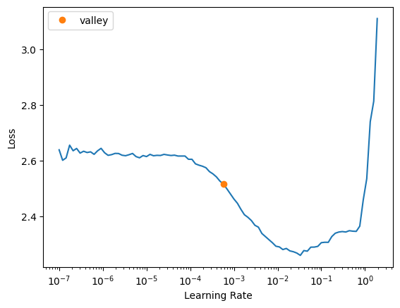

learn.loss_func

FlattenedLoss of CrossEntropyLoss()

wandb.init(
    project="tinyscale-lab",
    name="imagenette-xresnet34-bs-64-lr-1e-4",
)

learn = Learner(dls, xresnet34(n_out=10), metrics=accuracy, cbs=WandbCallback())
learn.fit_one_cycle(5, 1e-4)

epoch	train_loss	valid_loss	accuracy	time
0	2.054720	1.864616	0.371975	00:09
1	1.605212	1.489624	0.525350	00:09
2	1.307533	1.235453	0.619618	00:09
3	1.180410	1.153767	0.642038	00:09
4	1.124177	1.139668	0.644586	00:09

wandb.finish()

wandb.init(
    project="tinyscale-lab",
    name="imagenette-xresnet34-bs-64-lr-1e-3",
)

learn = Learner(dls, xresnet34(n_out=10), metrics=accuracy, cbs=WandbCallback())
learn.fit_one_cycle(5, 1e-3)

epoch	train_loss	valid_loss	accuracy	time
0	1.607826	1.416133	0.538344	00:10
1	1.204550	1.263326	0.578853	00:09
2	0.946661	0.917620	0.710828	00:09
3	0.784756	0.758046	0.755414	00:09
4	0.683072	0.704371	0.777580	00:09

wandb.finish()

wandb.init(
    project="tinyscale-lab",
    name="imagenette-xresnet34-bs-64-lr-1e-2",
)

learn = Learner(dls, xresnet34(n_out=10), metrics=accuracy, cbs=WandbCallback())
learn.fit_one_cycle(5, 1e-2)

epoch	train_loss	valid_loss	accuracy	time
0	1.571024	2.439970	0.335541	00:09
1	1.255883	2.097694	0.395414	00:09
2	1.018229	0.989576	0.681529	00:09
3	0.785577	0.728265	0.762293	00:09
4	0.623264	0.640818	0.792866	00:09

wandb.finish()

xresnet18

learn = Learner(dls, xresnet18(), metrics=accuracy)
learn.lr_find()

SuggestedLRs(valley=0.0020892962347716093)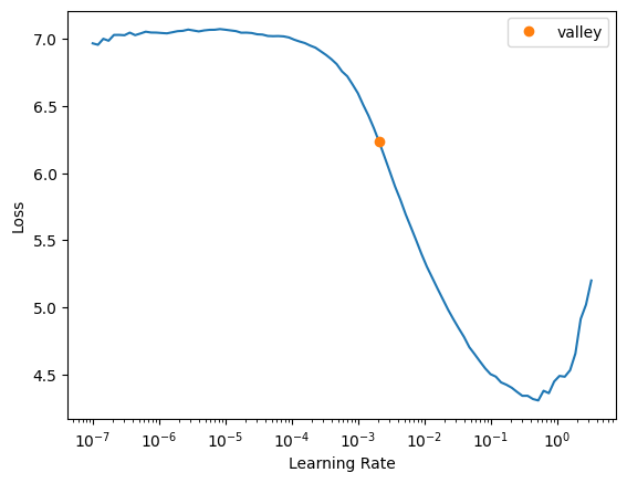

wandb.init(
    project="tinyscale-lab",
    name="imagenette-xresnet18-bs-64-lr-1e-4",
)

learn = Learner(dls, xresnet18(), metrics=accuracy, cbs=WandbCallback())
learn.fit_one_cycle(5, 1e-4)

epoch	train_loss	valid_loss	accuracy	time
0	5.608559	4.292247	0.301147	00:07
1	2.270526	1.728192	0.505478	00:07
2	1.517185	1.401804	0.579108	00:07
3	1.327132	1.287121	0.610446	00:07
4	1.274527	1.265958	0.617070	00:07

wandb.finish()

wandb.init(
    project="tinyscale-lab",
    name="imagenette-xresnet18-bs-64-lr-1e-3",
)

learn = Learner(dls, xresnet18(), metrics=accuracy, cbs=WandbCallback())
learn.fit_one_cycle(5, 1e-3)

epoch	train_loss	valid_loss	accuracy	time
0	2.134495	1.742504	0.445860	00:07
1	1.249879	1.266531	0.584204	00:07
2	0.986120	1.082811	0.648153	00:07
3	0.804976	0.767623	0.758471	00:07
4	0.708721	0.734305	0.774267	00:07

wandb.finish()

wandb.init(
    project="tinyscale-lab",
    name="imagenette-xresnet18-bs-64-lr-1e-2",
)

learn = Learner(dls, xresnet18(), metrics=accuracy, cbs=WandbCallback())
learn.fit_one_cycle(5, 1e-2)

epoch	train_loss	valid_loss	accuracy	time
0	1.665481	2.706135	0.358726	00:07
1	1.278437	1.516189	0.505987	00:07
2	1.017887	1.038873	0.663440	00:07
3	0.801989	0.718528	0.761529	00:07
4	0.638737	0.650084	0.787006	00:07

wandb.finish()

wandb.init(
    project="tinyscale-lab",
    name="imagenette-xresnet18-bs-64-lr-1e-1",
)

learn = Learner(dls, xresnet18(), metrics=accuracy, cbs=WandbCallback())
learn.fit_one_cycle(5, 1e-1)

epoch	train_loss	valid_loss	accuracy	time
0	1.755140	2.272295	0.325860	00:07
1	1.501531	3.738475	0.322293	00:07
2	1.238407	1.375671	0.547516	00:07
3	1.036412	0.896265	0.707516	00:07
4	0.850425	0.815597	0.737325	00:07

wandb.finish()