pip installs
!pip install transformers==4.49.0
!pip install ragatouille!pip install transformers==4.49.0
!pip install ragatouillefrom colbert.indexing.collection_encoder import CollectionEncoder
from colbert.infra import ColBERTConfig
from colbert.modeling.checkpoint import Checkpoint
from colbert.modeling.tokenization.utils import _split_into_batches, _sort_by_length, _insert_prefix_token
import random
import torch
from inspect import getsource
checkpoint = Checkpoint("answerdotai/answerai-colbert-small-v1", ColBERTConfig())
ce = CollectionEncoder(config=ColBERTConfig(), checkpoint=checkpoint)Instead of coming up with my own takeaways, I’m going to do something different this time, where I’m going to walk through Omar’s thread from 2023, where he himself summarizes the main takeaways from the ColBERT v1 paper.
Progress on dense retrievers is saturating.
— Omar Khattab (@lateinteraction) December 18, 2023
The best retrievers in 2024 will apply new forms of late interaction, i.e. scalable attention-like scoring for multi-vector embeddings.
A🧵on late interaction, how it works efficiently, and why/where it's been shown to improve quality pic.twitter.com/2XG33TtM9R
I think it’s important to highlight that he talks about new forms of late interaction as “scalable attention-like scoring for multi-vector embeddings”. From my understanding of ColBERT, the attention-like scoring mechanism refers to the BERT contextualization of meaning of tokens. As the query or the document goes through BERT, it passes through the attention mechanism, and tokens attend to each other. So no single query token or document token is isolated; it exists in the context of the entire query or the entire document that it’s in, respectively. The “multi-vector embeddings” part of his tweet is referring to this idea: we don’t compress an entire document or an entire query into a single vector, but instead have more than one vector representing different dimensions of meaning of the text.
Update: Omar clarified on Twitter that by “attention-like scoring mechanism” he was actually referring specifically to MaxSim as fast attention-like scoring, rather than the BERT contextualization during encoding that I initially described above. Which in hindsight makes sense—emphasis on “attention-like scoring mechanism”.
Say you have 1M documents. With infinite GPUs, what would your retriever look like?
— Omar Khattab (@lateinteraction) December 18, 2023
Maybe a cross-encoder? Finetune a large LM to take <query,doc> pairs. Run it 1M times to get a score for all docs.
Expressive! Given a query, the LM can pay attention to every detail in the doc! pic.twitter.com/P4t7bYe9dT
Something I want to highlight is that you still have to fine-tune a language model to become a retriever because the language model itself has this general knowledge about language and the relationship between words but it doesn’t have explicitly the capability of accurately producing a score that measures the relevancy of one body of text to another. So fine-tuning brings out that implicit skill that is in the latent space of the model into an actionable task. If we had infinite GPUs, we would want to get the relationship of every query token to every document token encoded. We would want to do this during training and we would want to do this during inference. That’s why he says “expressive” - this is the ultimate expressiveness or maximum expressiveness that you can achieve between query and document tokens. Your query tokens are no longer just contextualized within the query; they are contextualized within the query and every single document. That’s a really powerful expressive way of capturing meaning between two bodies of text to determine if they are related to each other to some level.
But cross-encoders are expensive: must re-run each doc thru the LM for every new query.
— Omar Khattab (@lateinteraction) December 18, 2023
Most retrievers are single-vector encoders: Cram each doc into a vector in advance; match queries/docs with a dot-product.
Scalable! We can apply dot-product search at the billion scale! pic.twitter.com/lvLp6vSd8K
On the other side of the spectrum, we have the least expressive encoding but it is also more scalable: single vector encoders. You’re cramming each document into a vector and then you’re matching the queries and documents with a dot product.
You’re getting limited contextualization because of the limited expressiveness of what the tokens mean because everything is expressed by a single vector. But this is the most scalable.
A huge burden on these bi-encoders: They must create one vector that captures every question you may ask about any content in the doc
— Omar Khattab (@lateinteraction) December 18, 2023
Repeatedly been shown to be really fragile (especially OOD) and data-inefficient.
Can we build far more effective, yet scalable, encoders?
I think the key here is that the motivation is not just to build more effective encoders but effective and scalable encoders.
A brief aside on the limitations of single vector representations.

There is a great talk by Antoine Chaffin published recently called “Late Interaction Beats Single Vectors for RAG Introduction to PyLate” which is part of Hamel Husain’s AI Evals course. He talks about how pooling is the intrinsic flaw of dense models: the pooling operation compresses n tokens into a single one, because of this selective behavior is learned during training through data, it gets more extreme with longer context because you have to compress more, and the compressed representation learns one notion of similarity. This is what Omar means by the “huge burden” on the bi-encoders. They have to compress a lot of information into a single representation.
If you think about it, during training, which Antoine is talking about here (and he also had a good thread on Twitter, which I can’t find because Twitter’s search is horrible) is that as you’re training a single vector representation, small changes in the query will result in wholesale changes of the single vector that represents the entire document.
So for example if you have a query about actors the document embedding will be trained on expressing that one notion of movies. If you have a separate query about the plot now the document encoding has to represent that different notion of similarity with one vector.
Antoine says in his thread that because of this you get a very noisy training experience for the document encodings because they’re constantly being tossed around left and right to match different notions of similarity with each query in the training step. They can’t match all of the notions because they are a single vector representation or compression of multiple tokens.
Contrast this with the late interaction setup where you have one representation for each token. Now, when you are training, the token embedding in the document that corresponds to the query about the actors gets modified and adjusted to result in a better relevance score. Later on in training, a query about the plot is going to activate the token in the document about the plot, and the query about the visual effects will activate the visual effect tokens in the document, and so on. So, you get this fine-grained, nuanced representation aligning with fine-grained, nuanced meaning in queries during training. The benefit of this is that n each step of training you can have a new, nuanced gradient update to the weights that produce these granular representations.
Back to Omar’s thread.
Late interaction (ColBERT) is simple.
— Omar Khattab (@lateinteraction) December 18, 2023
Let's not cram docs into a vector. Instead, let's make the attention (interaction) scalable.
How? Build a late interaction fn.
(1) Applied after, not during, encoding.
(2) Pruning-capable, i.e. scales better than linear. This is key! pic.twitter.com/m7fS15SdIE
If we want efficiency, we can’t get the full effect of attention. We can’t get all query tokens and all document tokens attending to each other. And we can get an interaction between query token embeddings and document token embeddings that is done efficiently if it is applied after, not during, encoding. The “late” in “late interaction” is what allows the pruning capability, which we’ll talk about later in the presentation.
Is there a function like this that preserves the retrieval precision of BERT attention?
— Omar Khattab (@lateinteraction) December 18, 2023
Oddly, yes and it's incredibly simple: just aggregate (sum) the MaxSim from query tokens to doc tokens.
Basically, softly locate each query vector in the doc (w dot product), and aggregate.
The key aspect of MaxSim is it takes the maximum similarity. Unlike something like average similarity, it doesn’t care about all tokens; it cares about the document token that has the maximum similarity with the given query token. This eliminates all but one document token from final consideration, which is what allows pruning capability to unlock. Because the interaction between query and document token embeddings happens after they’re encoded, you can encode queries and documents separately.
It was a last-ditch run on a Sunday night (3 Nov'19) after complex scoring failed.
— Omar Khattab (@lateinteraction) December 18, 2023
I spent weeks looking for a "bug". ColBERT w cheap scoring rivaled BERT-large cross-encoders with 10,000x more FLOPs?!
Called it ColBERT as a pun: late show / late interaction
log scale latency: pic.twitter.com/4MGmzAYHYG
Incredible that events like these happen, and I think happen quite frequently.
There's a little-known trick that was essential for ColBERT's results: Query Augmentation.
— Omar Khattab (@lateinteraction) December 18, 2023
ColBERT appends [MASK] tokens to the query encoder to allow BERT to create more query vectors that aren't there!
Is it the earliest form of a scratchpad / chain of thought? From Nov 2019! pic.twitter.com/2rIoMn1jxP
This is a super interesting concept that we’ll look at in detail later on.
As another aside—one of the reasons I was motivated to re-read the ColBERT V1 paper was this thread below by Antoine.
I am starting to be more and more convinced that MaxSim generalize very well to long documents but struggles on longer query, most probably due to the asymmetry
— Antoine Chaffin (@antoine_chaffin) July 9, 2025
Larger documents are bound by the number of query tokens, but larger queries might get noisy
Either it is a query…
If you have a document with 1k tokens and a query with 32 tokens, at most 32 document tokens will pass the maximum similarity threshold, hence “larger documents are bound by the number of query tokens.” As your query gets larger the meaning of tokens becomes diverse, this may create noise in the meaning expressed in the query. Query tokens with vastly different meanings will have maximum similarity with document tokens that are vastly different in meaning as well.
The conversation continues with:
Yes, that is also why it was not a big issue with query expansion because all the queries had the same number of tokens
— Antoine Chaffin (@antoine_chaffin) July 9, 2025
but with longer queries and no query exp, meh
slm tokens makes a really interesting point. Let’s assume that for each of the 32 query tokens, you find a document token that has a cosine similarity of 1. You add them up, and the maximum similarity is 32, the length of the query. That’s what they’re saying by the maximum MaxSim is the length of the query. Assuming that as your query gets longer, the meaning of the tokens starts to vary, and potentially the maximum similarity between the query and document tokens starts to vary.
You can imagine that you could have a very long query where one or more tokens are kind of obscure and may be on the fringes of the intent and meaning of the whole query, and potentially dissimilar to any document in the collection. These will potentially have a very small maximum similarity with some document token. In this situation, you can imagine that you have a very high variance because some query tokens will have high maximum similarities, some will have low, and you get this kind of noisy distribution of similarities across the query.
They go on to say that normalization can’t be something like the mean over query tokens, but has to be related to the distribution. Why does Antoine say that there is no query expansion? We’ll see that in the next tweet.
btw let's rule out query expansion because I am training models using flash attention and so there isn't any query expansion (I keep forgetting ffs 😭)
— Antoine Chaffin (@antoine_chaffin) July 9, 2025
This will make more sense after we look at query expansion/augmentation later in this blog post. Basically, query expansion relies on masked tokens containing semantic meaning, but, IIUC, Flash Attention negates masked tokens, so it nullifies the interaction between masked tokens and other tokens.
Here’s a tweet from Antoine 9 months ago that explains this:
Funny insight:
ColBERT query expansion works by adding tokens that are not attended but attend to the others
This works in the OG attention implementation with attention mask (as the attention values are computed for these tokens, their contributions are just masked out for the other tokens, but their representations are computed w.r.t the unmasked tokens)However, with Flash Attention, masked tokens embeddings are just zeros, meaning the contribution to MaxSim is always zeros and these tokens are not used, as if there was no query expansion at all
This might explain Jina-ColBERT results of attending vs not attending to those (which seems contrary to our results): if they activated FA during the tests, the comparaison is actually no query expansion vs query expansion with attending, not not attending vs attending — Antoine Chaffin (@antoine_chaffin) November 28, 2024
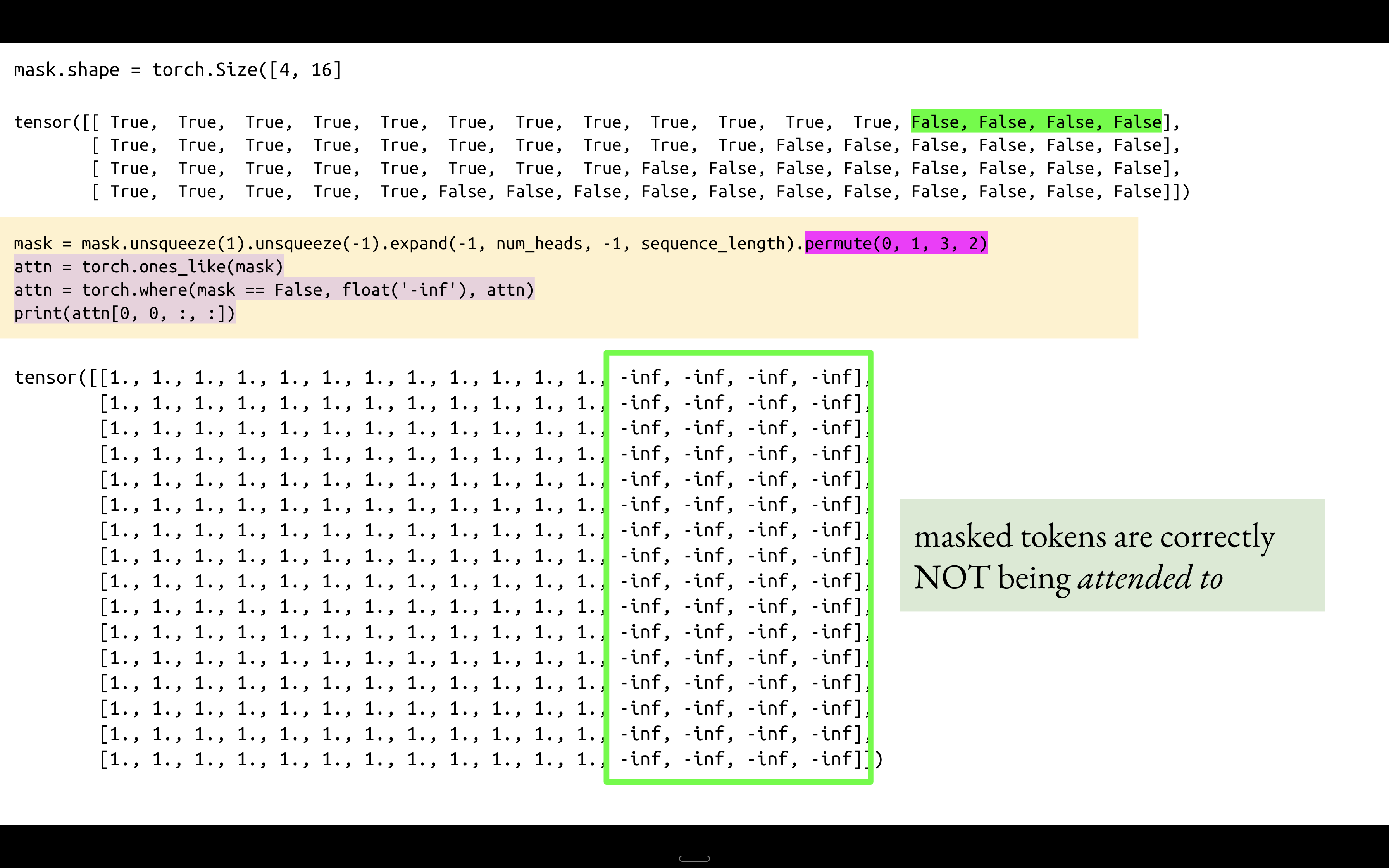
Here is a slide from a previous video that I made titled “Understanding Eager Bidirectional Attention via the Attention Mask”. In this case, we have 16 tokens, including four masked tokens. The large 16x16 tensor at the bottom is the attention scores tensor. The masked tokens are correctly not being attended to, but they do attend to other tokens. The last four columns are set to negative infinity because they are masked tokens, so their attention scores will be zero. But the last four rows do contain some 1s. The attention scores will not be zero for those rows and columns where we have 1s. Masked tokens are not being attended to, but they do attend to other tokens, and therefore they do have an attention score, and therefore they will have hidden states in the embedding space.
Back to Omar’s thread.
OK, but how can ColBERT search 100M docs in ~100 milliseconds?
— Omar Khattab (@lateinteraction) December 18, 2023
Late interaction is pruning-capable: it only needs to "touch" < 0.1% of the documents to find the top-K.
This is by design: it's composed of monotonic functions (Max/Sum), which enable some neat algorithmic tricks.
We can decompose late interaction into dozens of tiny nearest-neighbor searches, at the token level.
— Omar Khattab (@lateinteraction) December 18, 2023
We'll only fetch & score docs in which at least one token in close to (at least one token in) the query.
Otherwise, we can prove the score will be too small, and we can skip it! pic.twitter.com/6vBZp1U0Ku
As shown in the diagram, we have clusters of document token embeddings, clustered by some vector-similarity indexing process. For each query token embedding, we find the closest few clusters to it. We perform our MaxSim operation between the query tokens and all those clustered documents’ tokens. With this initial clustering step, we’re filtering out low-relevance documents using nearest neighbor search from the start.
With these main takeaways under our belt, in the following sections we’ll walk through each part of the ColBERTv1 paper in detail. I’ll provide excerpts from the paper in block quotes (highlighted emphasis mine) and then my thoughts after that.
To tackle this, we present ColBERT, a novel ranking model that adapts deep LMs (in particular, BERT) for efficient retrieval. ColBERT introduces a late interaction architecture that independently encodes the query and the document using BERT and then employs a cheap yet powerful interaction step that models their fine-grained similarity. By delaying and yet retaining this fine-granular interaction, ColBERT can leverage the expressiveness of deep LMs while simultaneously gaining the ability to pre-compute document representations offine, considerably speeding up query processing. Beyond reducing the cost of re-ranking the documents retrieved by a traditional model, ColBERT’s pruning-friendly interaction mechanism enables leveraging vector-similarity indexes for end-to-end retrieval directly from a large document collection. We extensively evaluate ColBERT using two recent passage search datasets. Results show that ColBERT’s effectiveness is competitive with existing BERT-based models (and outperforms every non-BERT baseline), while executing two orders-of-magnitude faster and requiring four orders-of-magnitude fewer FLOPs per query.
The key part about late interaction is that the architecture independently encodes the query and document. This allows you to index document representations offline which allows you to delay the query-document interaction until the end of the architecture.
What took me some unpacking is the line: > ColBERT’s pruning-friendly interaction mechanism enables leveraging vector-similarity indexes for end-to-end retrieval directly from a large document collection.
IIUC, the pruning-friendliness of ColBERT is unlocked by the fact that the interaction mechanism uses maximum similarity, and because of the nature of maximum (i.e. only 1 token can satisfy maximum) you can ignore low-similarity documents. Vector similarity indexes group together documents by similarity, so if a cluster of documents is not close to the query token embedding in question, it can be ignored completely.
On the terms “ranker” vs. “retriever” and what that brings up or me:
The terms Ranker and Retriever give me different mental images.
When I think of Ranker, I think of you already having some passages that are deemed relevant and you’re ranking them, bringing the best ones to the top.
When I think of Retriever, the mental image I have is that you have this collection of data documents, a corpus of text where you have irrelevant and relevant passages all mixed together. The retriever then goes in, sifts through this text, and finds the relevant passages.
It’s been a bit of an adjustment for me using these two as synonyms. So that’s something I just want to keep in mind as I’m reading literature is that Ranker and Retriever should give me the same mental image, but they don’t.
By computing deeply-contextualized semantic representations of query-document pairs, these LMs help bridge the pervasive vocabulary mismatch [21, 42] between documents and queries [30].
I wanted to highlight this sentence from the background section because I thought it was getting to the core of something about BERT that I didn’t really know. We’ll see in a bit. But first–
The following excerpt is from the paper Modeling and Solving Term Mismatch for Full-Text Retrieval Which is reference [42], written in 2012:
Even though modern retrieval systems typically use a multitude of features to rank documents, the backbone for search ranking is usually the standard tf.idf retrieval models.
This thesis addresses a limitation of the fundamental retrieval models, the term mismatch problem, which happens when query terms fail to appear in the documents that are relevant to the query. The term mismatch problem is a long standing problem in information retrieval.
I haven’t read the full thesis, but it does make sense that for keyword-based search, the query term failing to appear in the document that is relevant to the query would be a major problem as it’s frequency in the document would be 0.
Another paper referenced on this vocabulary mismatch problem is “Understanding the Behaviors of BERT and Ranking” where they say:
The observations suggest that, BERT’s pre-training on surrounding contexts favors text sequence pairs that are closer in their semantic meaning.
So, it seems like even in the embedding space, the term mismatch problem is present. Another excerpt from the same paper:
[BERT] prefers semantic matches between paraphrase tokens
Here’s Figure 2 from the same paper where each point on the chart corresponds to one query-passage pair with a random regular term removed from the passage:
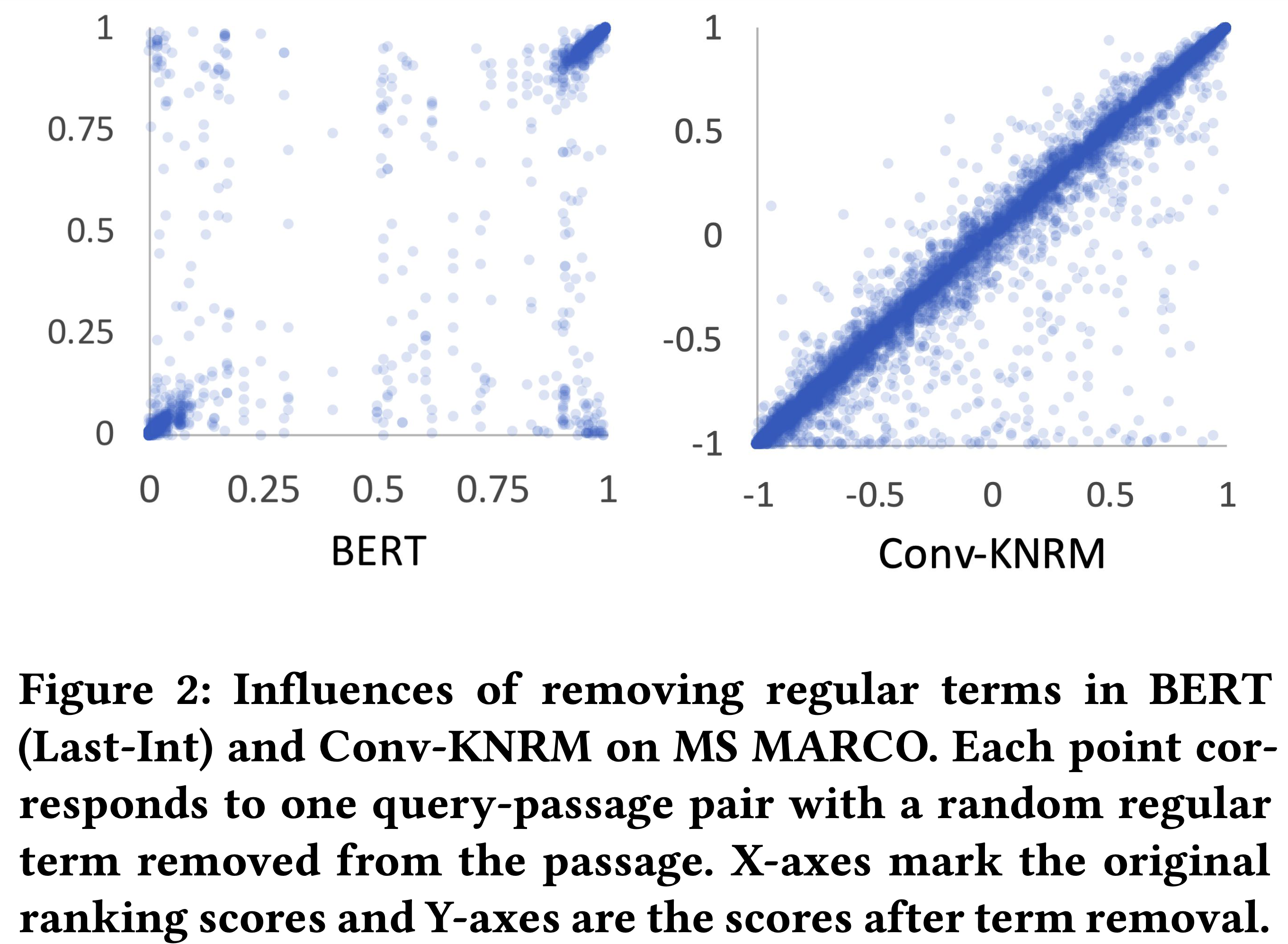
The x-axis is the original ranking score, and the y-axis is the score after the term is removed. One takeaway they had in the paper is that BERT in general has extreme scores. It either scores 1 or 0. But that’s not the main take away here when it comes to the concept of query-document-term mismatch. In the bottom right corner of the BERT chart, we can see that there are query-passage pairs with a high orginal ranking score and a low score after a term is removed. The original ranking of 1.0 drops to a ranking of 0.0. This is evidence that the query document term mismatch problem occurs in semantic space as well. If you remove a term that’s semantically similar in the query to the document, then BERT will not recognize the similarity between the two and will give the pair a low ranking score.
Let’s continue a little bit more into the background of neural rankers, but now in the context of how does ColBERT compare to these previous neural architectures?
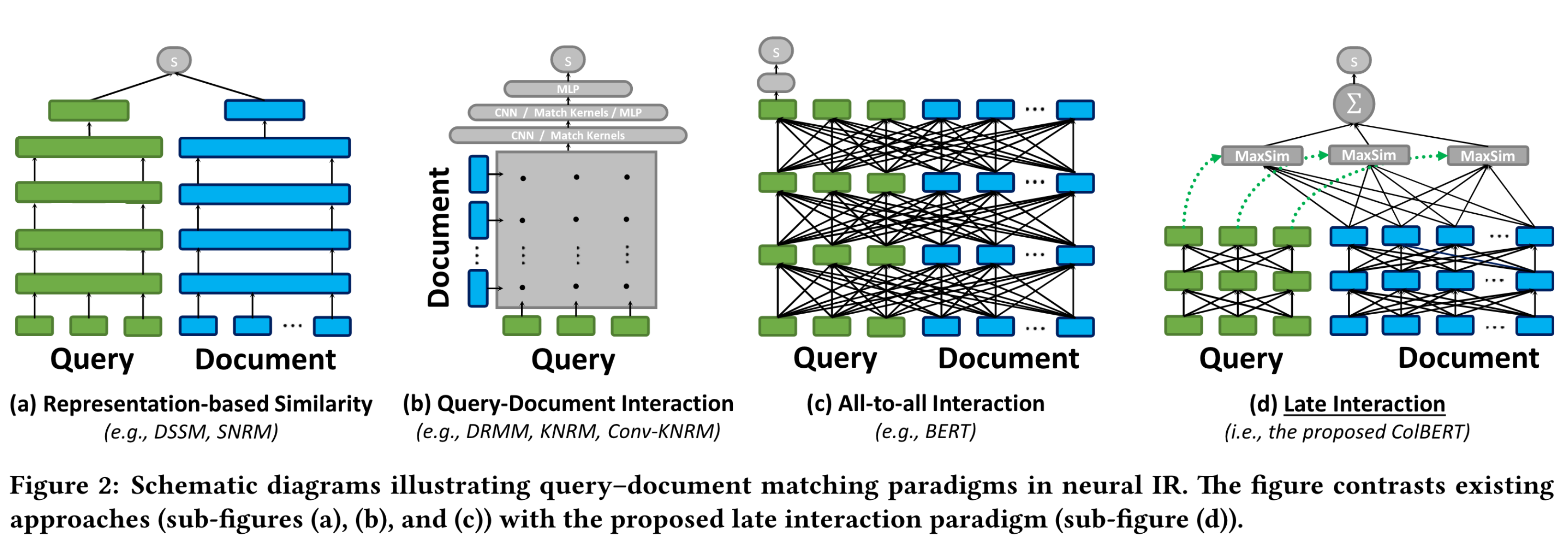
The small rectangles in this graphic represent words, subwords or tokens. The wider rectangle represent large dimension vectors or representations.
Representation-based Similarity (figure 2a) calculates a single cosine similarity score between a single query embedding and a single document embedding. Query-Document interaction (2b) feeds an interaction matrix with similarity scores between every pair of query-document tokens to a neural net which produces a single final similarity score. BERT (2c), all-to-all interaction, attends each token in the query to all other tokens in the query, and each token in the document to all other tokens in the document, contextualizing each token with all other query/document tokens. From the Passage Re-Ranking with BERT paper:
We use a BERT_LARGE model as a binary classification model, that is, we use the [CLS] vector as input to a single layer neural network to obtain the probability of the passage being relevant
Late interaction (2d), ColBERT, combines the best of both worlds: the offline computation of representation-based similarity and the richness/granularity of interaction-based similarity. Query tokens attend to each other during encoding, document tokens attend to each other during (offline) encoding; during interaction, each query token interacts with all document tokens and the document token with the maximum similarity is selected; these maximum similarities are summed across all query tokens, giving you one score per document. Not all documents in the collection need to be considered; vector similarity indexes naturally group relevant documents together. Searching for document token embeddings in clusters close to the query token embeddings reduces the number of candidates considered.
These architectural differences of ColBERT give it a ton of advantages:
As Figure 1 illustrates, ColBERT can serve queries in tens or few hundreds of milliseconds. For instance, when used for reranking as in “ColBERT (re-rank)”, it delivers over 170× speedup (and requires 14,000× fewer FLOPs) relative to existing BERT-based models, while being more effective than every non-BERT baseline (§4.2 & 4.3). ColBERT’s indexing—the only time it needs to feed documents through BERT—is also practical: it can index the MS MARCO collection of 9M passages in about 3 hours using a single server with four GPUs (§4.5), retaining its effectiveness with a space footprint of as little as few tens of GiBs.
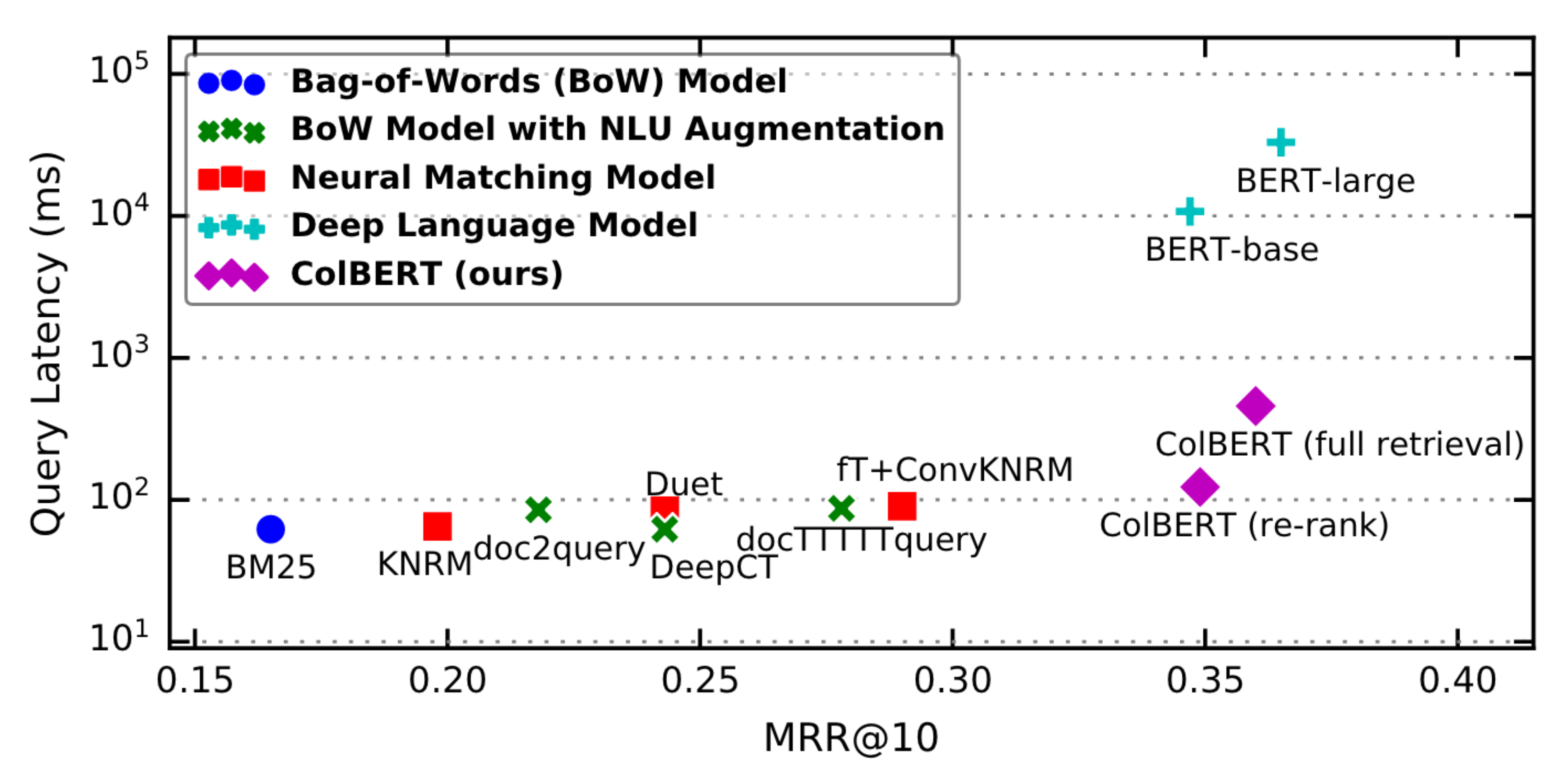
Figure 1 shows that ColBERT has comparable performance to BERT Large and BERT Base but a 100x faster query latency. This is not an insignificant difference, as they say that “raising query response times by as little as 100ms is known to impact user experience and even measurably diminish revenue”. So, it follows that a decrease from 10,000 milliseconds to 100s of milliseconds is going to measurably increase revenue.
One related paper I briefly want to focus on is this 2018 paper by Zamani et al, which introduces SNRM (emphasis mine):
In 2018, Zamani et al. [41] introduced SNRM, a representationfocused IR model that encodes each query and each document as a single, sparse high-dimensional vector of “latent terms”. By producing a sparse-vector representation for each document, SNRM is able to use a traditional IR inverted index for representing documents, allowing fast end-to-end retrieval. Despite highly promising results and insights, SNRM’s effectiveness is substantially outperformed by the state of the art on the datasets with which it was evaluated (e.g., see [18, 38]). While SNRM employs sparsity to allow using inverted indexes, we relax this assumption and compare a (dense) BERT-based representation-focused model against our late-interaction ColBERT in our ablation experiments
I fed the SNRM paper to Claude Sonnet 4 and asked it to give me an example of sparsity allows the use of an inverted file index:
Simple SNRM example:
Training produces latent terms like: - Latent term 47: “sports concepts” - Latent term 203: “technology concepts”
Document representations: - Doc A (about basketball): [0, 0, …, 0.8, 0, …, 0, 0, …] (high weight at position 47) - Doc B (about AI): [0, 0, …, 0, 0, …, 0.9, 0, …] (high weight at position 203)
Inverted index: - Latent term 47 → [Doc A: 0.8, Doc C: 0.3] - Latent term 203 → [Doc B: 0.9, Doc D: 0.5]
Query time: Sports query activates latent term 47 → quickly finds Doc A and C without checking every document.
Let’s say we have two document representations: document A which is about basketball and document B which is about AI. SNRM generates sparse representations, so a number of values are zero. Let’s say that we have a latent term 47 that’s about sports concepts and a latent term 203 that’s about technology concepts. The inverted index for latent term 47 is going to store the value of that term in doc A (which is 0.8) and in doc D (let’s say that’s 0.3). For the latent term 203 (which is technology concepts), the inverted index will store 0.9 for doc B (which is the highest position value) and 0.5 for doc D (which would be some relatively low position). At query time, a sports query activates the latent term for 47, and because that’s efficiently stored in the inverted index, it’s a quick lookup and you don’t have to check every document.
So now that we have a sense of where the ColBERT architecture falls in the context of previous work, we can now dive into the ColBERT architecture itself.
delaying the query–document interaction can facilitate cheap neural re-ranking (i.e., through pre-computation) and even support practical end-to-end neural retrieval (i.e., through pruning via vector-similarity search)
ColBERT balances neural retrieval quality and cost, benefiting both re-ranking and end-to-end retrieval. The delayed query-document interaction enables offline document indexing. At query time, you only encode the query and run MaxSim operations. For end-to-end retrieval, this same offline indexing allows vector similarity clustering—instead of searching all documents, you query the closest clusters, dramatically reducing candidates.
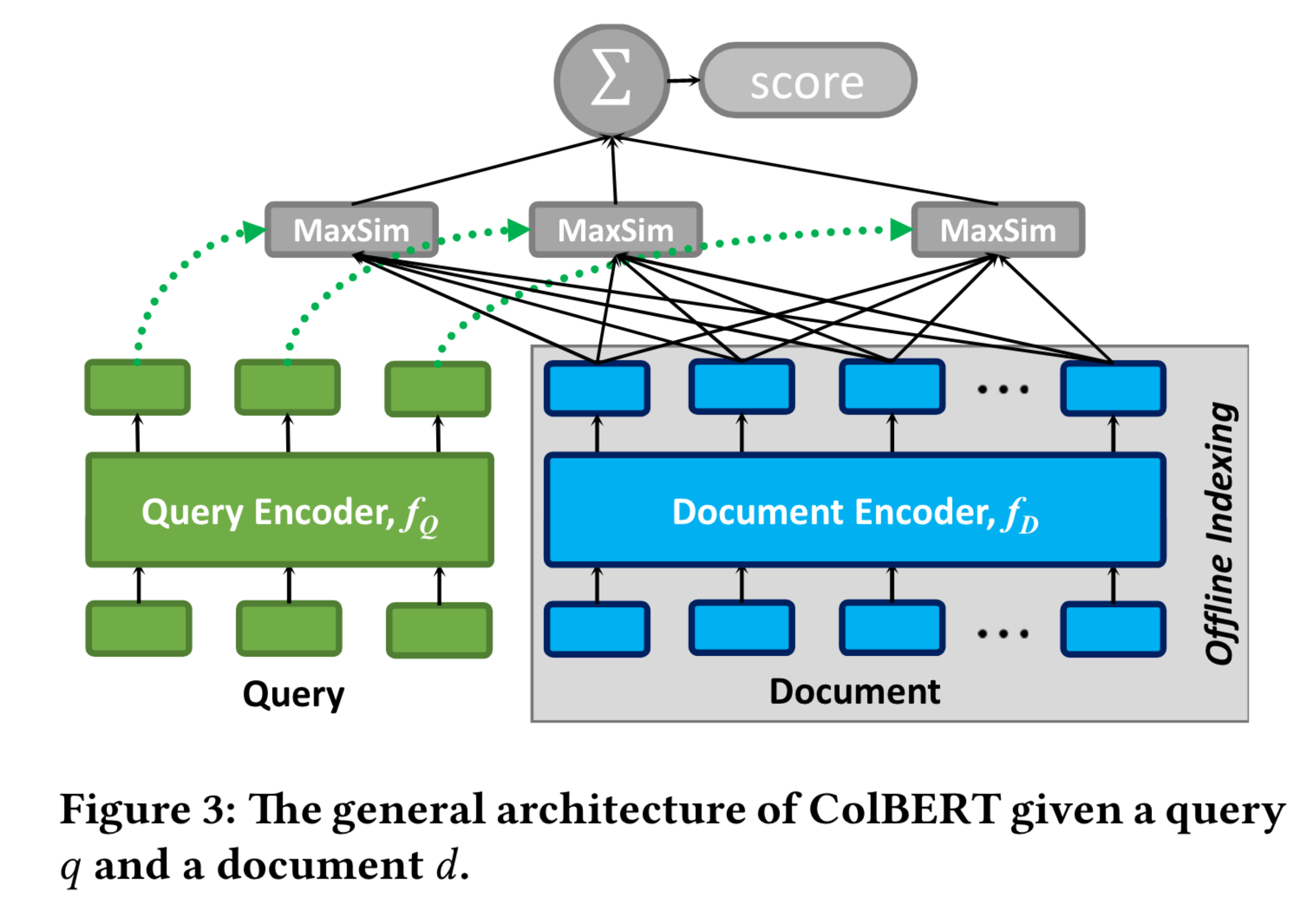
The general architecture of ColBERT, comprises of: a query encoder fQ (shown in green), a document encoder fD (shown in blue), and the late interaction mechanism S(shown in gray). Given a query q and document d, fQ encodes q into a bag of embeddings Eq while fD encodes d into another bag Ed. Each embeddings in Eq and Ed is contextualized based on the other terms in q or d, respectively.
Before we look at the Late Interaction Mechanism, let’s look closer at what is involved during the encoding of queries and documents.
We share a single BERT model among our query and document encoders but distinguish input sequences that correspond to queries and documents by prepending a special token [Q] to queries and another token [D] to documents.
Given BERT’s representation of each token, our encoder passes the contextualized output representations through a linear layer with no activations. This layer serves to control the dimension of ColBERT’s embeddings, producing m-dimensional embeddings for the layer’s output size m. As we discuss later in more detail, we typically x m to be much smaller than BERT’s xed hidden dimension.
While ColBERT’s embedding dimension has limited impact on the efficiency of query encoding, this step is crucial for controlling the space footprint of documents
A quick note about embedding dimension: there are models such as answerai-colbert-small-v1 where the embedding dimension is as small as 96.
Here’s the desription of the query encoder:
Query Encoder. Given a textual query q, we tokenize it into its BERT-based WordPiece [35] tokens q1, q2…ql . We prepend the token [Q] to the query. We place this token right after BERT’s sequence-start token [CLS]. If the query has fewer than a pre-defined number of tokens Nq , we pad it with BERT’s special [mask] tokens up to length Nq (otherwise, we truncate it to the first Nq tokens). This padded sequence of input tokens is then passed into BERT’s deep transformer architecture, which computes a contextualized representation of each token.
Here is a key contribution of this paper, that I am going to do a dive into next:
We denote the padding with masked tokens as query augmentation, a step that allows BERT to produce query-based embeddings at the positions corresponding to these masks. Query augmentation is intended to serve as a soft, differentiable mechanism for learning to expand queries with new terms or to re-weigh existing terms based on their importance for matching the query. As we show in §4.4, this operation is essential for ColBERT’s effectiveness.
Query augmentation is the idea that mask tokens carry semantic meaning, so padding short queries up to some fixed length expands the queries with these new semantically relevant terms, adding more nuance to help match similar terms in documents. In this side quest, I want to understand just how semantically similar these mask token embeddings are to the non-mask query tokens. I’ll start by digging into the code in the repo which takes text and converts it to embeddings.
Here’s how the Searcher encodes the query, where it uses queryFromText
def encode(self, text: TextQueries, full_length_search=False):
    queries = text if type(text) is list else [text]
    bsize = 128 if len(queries) > 128 else None

    self.checkpoint.query_tokenizer.query_maxlen = self.config.query_maxlen
    Q = self.checkpoint.queryFromText(queries, bsize=bsize, to_cpu=True, full_length_search=full_length_search)

    return Q
checkpoint.query_tokenizer.query_maxlen = 32
Q = checkpoint.queryFromText(["this is a short query"], bsize=1, to_cpu=True, full_length_search=False)/usr/local/lib/python3.11/dist-packages/colbert/utils/amp.py:15: FutureWarning: `torch.cuda.amp.autocast(args...)` is deprecated. Please use `torch.amp.autocast('cuda', args...)` instead.
return torch.cuda.amp.autocast() if self.activated else NullContextManager()Q.shapetorch.Size([1, 32, 96])Note that even though there are less than 32 tokens in "this is a short query", the norm of all Q embeddings is 1.0. This is because ColBERT adds [MASK] tokens to pad the query to a 32-token length, which we’ll see next.
Q.norm(dim=2)tensor([[1.0000, 1.0000, 1.0000, 1.0000, 1.0000, 1.0000, 1.0000, 1.0000, 1.0000,
1.0000, 1.0000, 1.0000, 1.0000, 1.0000, 1.0000, 1.0000, 1.0000, 1.0000,
1.0000, 1.0000, 1.0000, 1.0000, 1.0000, 1.0000, 1.0000, 1.0000, 1.0000,
1.0000, 1.0000, 1.0000, 1.0000, 1.0000]])checkpoint.queryFromText uses QueryTokenizer.tokenizer which does the following:
It first tokenizes the text
# tokenize with max_length - 1 to add the marker id afterwards
obj = self.tok(batch_text, padding='max_length', truncation=True,
                return_tensors='pt', max_length=(max_length - 1)).to(DEVICE)

ids = _insert_prefix_token(obj['input_ids'], self.Q_marker_token_id)
mask = _insert_prefix_token(obj['attention_mask'], 1)
And then replaces the padding token with the mask token.
# postprocess for the [MASK] augmentation
ids[ids == self.pad_token_id] = self.mask_token_id
Looking at that concretely:
obj = checkpoint.query_tokenizer.tok(["this is a short query"], padding='max_length', truncation=True,
                return_tensors='pt', max_length=(32 - 1))

ids = _insert_prefix_token(obj['input_ids'], checkpoint.query_tokenizer.Q_marker_token_id)
mask = _insert_prefix_token(obj['attention_mask'], 1)idstensor([[ 101, 1, 2023, 2003, 1037, 2460, 23032, 102, 0, 0,
0, 0, 0, 0, 0, 0, 0, 0, 0, 0,
0, 0, 0, 0, 0, 0, 0, 0, 0, 0,
0, 0]])ids[ids == checkpoint.query_tokenizer.pad_token_id] = checkpoint.query_tokenizer.mask_token_id
idstensor([[ 101, 1, 2023, 2003, 1037, 2460, 23032, 102, 103, 103,
103, 103, 103, 103, 103, 103, 103, 103, 103, 103,
103, 103, 103, 103, 103, 103, 103, 103, 103, 103,
103, 103]])checkpoint.query_tokenizer.tok.decode([103])'[MASK]'checkpoint.query_tokenizer.tok.decode(ids[0])'[CLS] [unused0] this is a short query [SEP] [MASK] [MASK] [MASK] [MASK] [MASK] [MASK] [MASK] [MASK] [MASK] [MASK] [MASK] [MASK] [MASK] [MASK] [MASK] [MASK] [MASK] [MASK] [MASK] [MASK] [MASK] [MASK] [MASK] [MASK]'This replacement of pad tokens with mask tokens is critical because queryFromText calls query which is defined as:
 def query(self, input_ids, attention_mask):
    input_ids, attention_mask = input_ids.to(self.device), attention_mask.to(self.device)
    Q = self.bert(input_ids, attention_mask=attention_mask)[0]
    Q = self.linear(Q)

    mask = torch.tensor(self.mask(input_ids, skiplist=[]), device=self.device).unsqueeze(2).float()
    Q = Q * mask

    return torch.nn.functional.normalize(Q, p=2, dim=2)
It actually creates its own mask to multiply Q by—it doesn’t use attention_mask.
Looking at mask:
print(getsource(checkpoint.mask)) def mask(self, input_ids, skiplist):
mask = [[(x not in skiplist) and (x != self.pad_token) for x in d] for d in input_ids.cpu().tolist()]
return mask
If the token is not in skiplist and != self.pad_token it gets a 1 in the mask. Since we swapped pad tokens with MASK tokens, they get a 1.
idstensor([[ 101, 1, 2023, 2003, 1037, 2460, 23032, 102, 103, 103,
103, 103, 103, 103, 103, 103, 103, 103, 103, 103,
103, 103, 103, 103, 103, 103, 103, 103, 103, 103,
103, 103]])torch.tensor(checkpoint.mask(ids, skiplist=[])).float()tensor([[1., 1., 1., 1., 1., 1., 1., 1., 1., 1., 1., 1., 1., 1., 1., 1., 1., 1.,
1., 1., 1., 1., 1., 1., 1., 1., 1., 1., 1., 1., 1., 1.]])As we can see, the mask is all 1s, so Q remains unchanged.
As an aside, I’ve been thinking about how RAGatouille sets the maximum query length based on the full query length (instead of fixing to 32):
if isinstance(query, str):
    query_length = int(len(query.split(" ")) * 1.35)
    self._upgrade_searcher_maxlen(query_length, base_model_max_tokens)
    results = [self._search(query, k, pids)]
else:
    longest_query_length = max([int(len(x.split(" ")) * 1.35) for x in query])
    self._upgrade_searcher_maxlen(longest_query_length, base_model_max_tokens)
    results = self._batch_search(query, k)
I think the following note about full_length_search in the ColBERT repo is related but I’m not currently sure:
# Full length search is only available for single inference (for now)
# Batched full length search requires far deeper changes to the code base
assert(full_length_search == False or (type(batch_text) == list and len(batch_text) == 1))

if full_length_search:
    # Tokenize each string in the batch
    un_truncated_ids = self.tok(batch_text, add_special_tokens=False).to(DEVICE)['input_ids']
    # Get the longest length in the batch
    max_length_in_batch = max(len(x) for x in un_truncated_ids)
    # Set the max length
    max_length = self.max_len(max_length_in_batch)
else:
    # Max length is the default max length from the config
    max_length = self.query_maxlen
MASK token embeddings are not meaninglessSo what meaning is embedded for the MASK token in the semantic space? To (lightly) explore this, I’ll calculate the cosine similarity between the non-MASK and MASK tokens.
ids[0][:7]tensor([ 101, 1, 2023, 2003, 1037, 2460, 23032])checkpoint.query_tokenizer.tok.decode(ids[0][:7])'[CLS] [unused0] this is a short query'checkpoint.query_tokenizer.tok.decode([2460, 23032])'short query'ids[0][8:]tensor([103, 103, 103, 103, 103, 103, 103, 103, 103, 103, 103, 103, 103, 103,
103, 103, 103, 103, 103, 103, 103, 103, 103, 103])checkpoint.query_tokenizer.tok.decode(ids[0][8:])'[MASK] [MASK] [MASK] [MASK] [MASK] [MASK] [MASK] [MASK] [MASK] [MASK] [MASK] [MASK] [MASK] [MASK] [MASK] [MASK] [MASK] [MASK] [MASK] [MASK] [MASK] [MASK] [MASK] [MASK]'Gathering the 96-dimensional embeddings for my non-MASK tokens.
Qnm = Q[0][:7]
Qnm.shape, Qnm.unsqueeze(0).shape
(torch.Size([7, 96]), torch.Size([1, 7, 96]))Gathering the 96-dimensional embeddings for my MASK tokens.
Qm = Q[0][7:]
Qm.shape, Qm.unsqueeze(1).shape
(torch.Size([25, 96]), torch.Size([25, 1, 96]))Taking the cosine similarity between the non-MASK and MASK tokens, we see that the MASK tokens (rows) are considerably similar in meaning (and in one case exactly the same) to the non-MASK tokens (columns)!
torch.nn.functional.cosine_similarity(Qnm.unsqueeze(0), Qm.unsqueeze(1), dim=2)tensor([[1.0000, 0.9709, 0.9150, 0.9461, 0.9672, 0.7417, 0.6532],
[0.9793, 0.9566, 0.9038, 0.9301, 0.9495, 0.7177, 0.6400],
[0.9804, 0.9585, 0.9053, 0.9320, 0.9517, 0.7195, 0.6380],
[0.9814, 0.9604, 0.9059, 0.9340, 0.9534, 0.7198, 0.6394],
[0.9812, 0.9598, 0.9065, 0.9342, 0.9533, 0.7220, 0.6390],
[0.9814, 0.9601, 0.9073, 0.9355, 0.9537, 0.7223, 0.6341],
[0.9816, 0.9612, 0.9068, 0.9367, 0.9549, 0.7222, 0.6354],
[0.9809, 0.9604, 0.9050, 0.9357, 0.9535, 0.7212, 0.6333],
[0.9823, 0.9623, 0.9064, 0.9385, 0.9562, 0.7228, 0.6365],
[0.9826, 0.9629, 0.9070, 0.9389, 0.9567, 0.7249, 0.6373],
[0.9818, 0.9614, 0.9062, 0.9387, 0.9554, 0.7248, 0.6390],
[0.9819, 0.9608, 0.9044, 0.9387, 0.9550, 0.7241, 0.6388],
[0.9821, 0.9620, 0.9032, 0.9394, 0.9561, 0.7252, 0.6372],
[0.9830, 0.9655, 0.9048, 0.9428, 0.9601, 0.7278, 0.6390],
[0.9836, 0.9690, 0.9081, 0.9459, 0.9632, 0.7273, 0.6392],
[0.9860, 0.9761, 0.9165, 0.9517, 0.9717, 0.7343, 0.6475],
[0.9850, 0.9848, 0.9299, 0.9542, 0.9805, 0.7550, 0.6576],
[0.9805, 0.9872, 0.9360, 0.9545, 0.9827, 0.7667, 0.6658],
[0.9780, 0.9878, 0.9385, 0.9544, 0.9833, 0.7705, 0.6693],
[0.9774, 0.9879, 0.9389, 0.9543, 0.9832, 0.7701, 0.6699],
[0.9764, 0.9887, 0.9397, 0.9549, 0.9839, 0.7709, 0.6731],
[0.9762, 0.9887, 0.9394, 0.9548, 0.9838, 0.7714, 0.6736],
[0.9763, 0.9885, 0.9396, 0.9548, 0.9837, 0.7715, 0.6738],
[0.9776, 0.9881, 0.9392, 0.9551, 0.9837, 0.7709, 0.6713],
[0.9772, 0.9887, 0.9400, 0.9555, 0.9840, 0.7714, 0.6736]])It’s interesting to note that the first MASK token (first row) has a cosine similarity of 1 with the first non-MASK token (the [CLS] tokens, first column). Other interesting observations:
[unused0], second column) is more similar to the last MASK token than most of the other MASK tokens.short query, 6th and 7th columns) than they are to the first five non-MASK tokens.I think this is enough evidence to show that the MASK tokens carry semantic meaning important to the query.
Returning to the paper, let’s see what they have to say about the document encoder:
Document Encoder. Our document encoder has a very similar architecture. We first segment a document d into its constituent tokens d1, d2…dm, to which we prepend BERT’s start token [CLS] followed by our special token [D] that indicates a document sequence. Unlike queries, we do not append [mask] tokens to documents. After passing this input sequence through BERT and the subsequent linear layer, the document encoder filters out the embeddings corresponding to punctuation symbols, determined via a pre-defined list. This filtering is meant to reduce the number of embeddings per document, as we hypothesize that (even contextualized) embeddings of punctuation are unnecessary for effectiveness. In summary, given q = q0, q1…ql and d = d0, d1…dn , we compute the bags of embeddings Eq and Ed in the following manner, where # refers to the [mask] tokens:
Eq := Normalize( CNN( BERT(“[Q]q0q1…ql ##…#”) ) ) (1)
Ed := Filter( Normalize( CNN( BERT(“[D]d0d1…dn”) ) ) ) (2)
I want to highlight something they say about how they encode their documents:
When batching, we pad all documents to the maximum length of a document within the batch. To make capping the sequence length on a per-batch basis more effective, our indexer proceeds through documents in groups of B (e.g., B = 100,000) documents. It sorts these documents by length and then feeds batches of b (e.g., b = 128) documents of comparable length through our encoder.
So let’s look at some of the code. In the CollectionEncoder class, which is what’s used to encode documents and queries, they call docFromText and they pass to it the passages which are currently strings:
for passages_batch in batch(passages, self.config.index_bsize * 50):
    embs_, doclens_ = self.checkpoint.docFromText(
        passages_batch,
        ...)
Inside docFromText, the document tokenizer’s tensorize method is called, and you pass to it the documents which are still strings:
if bsize:
    text_batches, reverse_indices = self.doc_tokenizer.tensorize(
        docs, bsize=bsize
    )
And then inside DocTokenizer.tensorize, you first convert the text into tokens. And then you pass those tokens into the _sort_by_length helper method:
def tensorize(self, batch_text, bsize=None):
    assert type(batch_text) in [list, tuple], (type(batch_text))

    obj = self.tok(batch_text, padding='longest', truncation='longest_first',
                    return_tensors='pt', max_length=(self.doc_maxlen - 1)).to(DEVICE)

    ids = _insert_prefix_token(obj['input_ids'], self.D_marker_token_id)
    mask = _insert_prefix_token(obj['attention_mask'], 1)

    if bsize:
        ids, mask, reverse_indices = _sort_by_length(ids, mask, bsize)
        batches = _split_into_batches(ids, mask, bsize)
        return batches, reverse_indices

    return ids, mask
And finally, inside the _sort_by_length method, it sums the mask in the last dimension, which is the sequence length dimension. Then it sorts it, grabs those indices, and returns the tokens of the passages in order. Using those indices:
def _sort_by_length(ids, mask, bsize):
    if ids.size(0) <= bsize:
        return ids, mask, torch.arange(ids.size(0))

    indices = mask.sum(-1).sort().indices
    reverse_indices = indices.sort().indices

    return ids[indices], mask[indices], reverse_indices
They’re summing the mask across the sequence length dimension (mask.sum(-1)). The mask contains 1s where you have non-padding tokens and 0s where you have padding tokens. So the sum of the mask across a sequence is the number of non-padding tokens in it. Sorting by this sum sorts the sequences by non-padding token length in ascending order.
Let’s look at this concretely through code.
To better understand how ColBERT sorts documents by length for batching, I’m going to walk through a toy example using the internal methods provided in the repo.
I’ll start by intentionally creating a list of passages of four different lengths: 40, 60, 80, and 100
passages = []
for i in range(128):
    if i < 32: passages.append("a " * 100)
    if i >= 32 and i < 64: passages.append("a " * 80)
    if i >= 64 and i < 96: passages.append("a " * 60)
    if i >= 96: passages.append("a " * 40)
I now pass the passages with a bat size of 32 into the Checkpoints.DocFromText method, and as a result, I get encoded documents where the bat size is 128, the maximum document length is 103, and the embedding dimension is 96 because I’m using answerai-colbert-small-v1.
res = ce.checkpoint.docFromText(docs=passages, bsize=32)/usr/local/lib/python3.11/dist-packages/colbert/utils/amp.py:15: FutureWarning: `torch.cuda.amp.autocast(args...)` is deprecated. Please use `torch.amp.autocast('cuda', args...)` instead.
return torch.cuda.amp.autocast() if self.activated else NullContextManager()res[0].shapetorch.Size([128, 103, 96])If we look one level deeper, inside docfromtext it calls the docTokenizer’s tensorize method which converts the string of text into tokens
text_batches, reverse_indices = ce.checkpoint.doc_tokenizer.tensorize(passages, bsize=32)text_batches[0][0].shapetorch.Size([32, 103])text_batches[0][0][0]tensor([ 101, 2, 1037, 1037, 1037, 1037, 1037, 1037, 1037, 1037, 1037, 1037,
1037, 1037, 1037, 1037, 1037, 1037, 1037, 1037, 1037, 1037, 1037, 1037,
1037, 1037, 1037, 1037, 1037, 1037, 1037, 1037, 1037, 1037, 1037, 1037,
1037, 1037, 1037, 1037, 1037, 1037, 102, 0, 0, 0, 0, 0,
0, 0, 0, 0, 0, 0, 0, 0, 0, 0, 0, 0,
0, 0, 0, 0, 0, 0, 0, 0, 0, 0, 0, 0,
0, 0, 0, 0, 0, 0, 0, 0, 0, 0, 0, 0,
0, 0, 0, 0, 0, 0, 0, 0, 0, 0, 0, 0,
0, 0, 0, 0, 0, 0, 0], device='cuda:0')Taking a look at the number of tokens in each of the batch items.
for i in [0, 32, 64, 96]:
    obj = ce.checkpoint.doc_tokenizer.tok(passages[i], padding='longest', truncation='longest_first',
                       return_tensors='pt', max_length=(ce.checkpoint.doc_tokenizer.doc_maxlen - 1))
    print(obj['input_ids'].shape)
torch.Size([1, 102])
torch.Size([1, 82])
torch.Size([1, 62])
torch.Size([1, 42])tensorize adds the [Q] or [D] token, so that’s why the first batch item only has 102 tokens, whereas after Tensorize, it has 103 tokens.
Before I run the rest of the sorting code, I’m going to shuffle the passages so that we can see if sorting actually takes place.
random.shuffle(passages)for o in passages[:10]: print(len(o))80
120
80
80
160
80
160
160
120
200When passing all of the passages to the .tok method, the tokenized batch has a number of tokens equal to the largest, longest passage. All 128 passages are tokenized up to a length of 102.
obj = ce.checkpoint.doc_tokenizer.tok(passages, padding='longest', truncation='longest_first',
                       return_tensors='pt', max_length=(ce.checkpoint.doc_tokenizer.doc_maxlen - 1))
obj['input_ids'].shape
torch.Size([128, 102])Here’s the step where we add the prefixed tokens for the documents, which is [D].
ids = _insert_prefix_token(obj['input_ids'], ce.checkpoint.doc_tokenizer.D_marker_token_id)
mask = _insert_prefix_token(obj['attention_mask'], 1)
ids.shape, mask.shape(torch.Size([128, 103]), torch.Size([128, 103]))Looking at the number of non-zero tokens in the batch (i.e., the non-padding tokens), we can see that our batch is still currently unsorted
for i in range(10):
    print(torch.count_nonzero(ids[i]))
tensor(43)
tensor(63)
tensor(43)
tensor(43)
tensor(83)
tensor(43)
tensor(83)
tensor(83)
tensor(63)
tensor(103)Looking at the sum of the masks, we can see that the sum of masks is equal to the number of non-padding tokens in the batch item.
for i in range(10): print(sum(mask[i]))tensor(43)
tensor(63)
tensor(43)
tensor(43)
tensor(83)
tensor(43)
tensor(83)
tensor(83)
tensor(63)
tensor(103)Alright, here’s the main part where it sorts by length the batches.
ids, mask, reverse_indices = _sort_by_length(ids, mask, bsize=32)
ids.shape, mask.shape
(torch.Size([128, 103]), torch.Size([128, 103]))Looking at the lengths of non-zero values in ids and mask. The items are now sorted by token length in increasing order.
for i in range(10):
    print(torch.count_nonzero(ids[i]), sum(mask[i]))
tensor(43) tensor(43)
tensor(43) tensor(43)
tensor(43) tensor(43)
tensor(43) tensor(43)
tensor(43) tensor(43)
tensor(43) tensor(43)
tensor(43) tensor(43)
tensor(43) tensor(43)
tensor(43) tensor(43)
tensor(43) tensor(43)It then splits it into batches of 32. Note that all batches are padded up to the maximum document length.
batches = _split_into_batches(ids, mask, bsize=32)for i in range(4): print(batches[i][0].shape)torch.Size([32, 103])
torch.Size([32, 103])
torch.Size([32, 103])
torch.Size([32, 103])Looking at the lengths of non-zero values in each batch we can see that the batches are now sorted by length of passage.
for i in range(4):
print(f"------ Batch {i}")
for j in range(10):
print(torch.count_nonzero(batches[i][0][j]), sum(batches[i][1][j]))------ Batch 0
tensor(43) tensor(43)
tensor(43) tensor(43)
tensor(43) tensor(43)
tensor(43) tensor(43)
tensor(43) tensor(43)
tensor(43) tensor(43)
tensor(43) tensor(43)
tensor(43) tensor(43)
tensor(43) tensor(43)
tensor(43) tensor(43)
------ Batch 1
tensor(63) tensor(63)
tensor(63) tensor(63)
tensor(63) tensor(63)
tensor(63) tensor(63)
tensor(63) tensor(63)
tensor(63) tensor(63)
tensor(63) tensor(63)
tensor(63) tensor(63)
tensor(63) tensor(63)
tensor(63) tensor(63)
------ Batch 2
tensor(83) tensor(83)
tensor(83) tensor(83)
tensor(83) tensor(83)
tensor(83) tensor(83)
tensor(83) tensor(83)
tensor(83) tensor(83)
tensor(83) tensor(83)
tensor(83) tensor(83)
tensor(83) tensor(83)
tensor(83) tensor(83)
------ Batch 3
tensor(103) tensor(103)
tensor(103) tensor(103)
tensor(103) tensor(103)
tensor(103) tensor(103)
tensor(103) tensor(103)
tensor(103) tensor(103)
tensor(103) tensor(103)
tensor(103) tensor(103)
tensor(103) tensor(103)
tensor(103) tensor(103)Now let’s go a layer deeper and look at _sort_by_length to see how the sorting actually happens. I’ll reinstantiate the passages and shuffle them to make sure the sorting actually happens.
passages = []
for i in range(128):
    if i < 32: passages.append("a " * 100)
    if i >= 32 and i < 64: passages.append("a " * 80)
    if i >= 64 and i < 96: passages.append("a " * 60)
if i >= 96: passages.append("a " * 40)random.shuffle(passages)I’ll also tokenize the passages and insert the prefix tokens.
obj = ce.checkpoint.doc_tokenizer.tok(passages, padding='longest', truncation='longest_first',
                       return_tensors='pt', max_length=(ce.checkpoint.doc_tokenizer.doc_maxlen - 1))
obj['input_ids'].shape
torch.Size([128, 102])ids = _insert_prefix_token(obj['input_ids'], ce.checkpoint.doc_tokenizer.D_marker_token_id)
mask = _insert_prefix_token(obj['attention_mask'], 1)ids.shape, mask.shape(torch.Size([128, 103]), torch.Size([128, 103]))Checking to make sure that my batch is shuffled
for i in range(10):
    print(torch.count_nonzero(ids[i]))
tensor(103)
tensor(103)
tensor(43)
tensor(83)
tensor(83)
tensor(103)
tensor(63)
tensor(83)
tensor(43)
tensor(43)To sort the batch items by length of non-padding tokens, they sum the mask across the last dimension, which is the number of tokens.
mask.shapetorch.Size([128, 103])So, what you get here is basically the number of non-padding tokens in each of the 128 items.
mask.sum(-1)tensor([103, 103, 43, 83, 83, 103, 63, 83, 43, 43, 103, 83, 43, 83,
63, 83, 43, 103, 43, 63, 103, 103, 43, 43, 103, 63, 83, 103,
103, 103, 103, 63, 43, 83, 63, 83, 63, 103, 43, 43, 63, 63,
103, 43, 103, 43, 63, 103, 43, 43, 63, 63, 83, 63, 103, 103,
83, 63, 103, 83, 43, 103, 103, 63, 83, 43, 103, 83, 83, 103,
103, 63, 63, 83, 43, 83, 83, 43, 83, 43, 103, 83, 103, 43,
83, 83, 43, 63, 63, 63, 103, 63, 43, 103, 83, 63, 63, 43,
63, 103, 83, 83, 83, 103, 63, 63, 63, 83, 83, 43, 43, 63,
103, 83, 63, 83, 43, 83, 63, 63, 43, 43, 43, 63, 103, 43,
83, 43])Then they sort it and get the indices.
indices = mask.sum(-1).sort().indices
indices
tensor([ 49, 22, 23, 110, 109, 32, 38, 43, 45, 48, 39, 97, 60, 92,
65, 86, 83, 74, 79, 77, 121, 127, 2, 125, 122, 8, 9, 116,
120, 12, 18, 16, 63, 51, 53, 98, 96, 57, 95, 25, 114, 91,
31, 89, 6, 88, 87, 123, 71, 72, 19, 119, 34, 106, 36, 105,
14, 50, 40, 41, 104, 118, 46, 111, 64, 107, 126, 81, 108, 115,
84, 85, 94, 102, 101, 113, 117, 100, 15, 33, 35, 26, 52, 56,
59, 13, 11, 7, 67, 76, 78, 75, 3, 73, 4, 68, 17, 1,
20, 21, 24, 124, 112, 27, 28, 29, 10, 5, 93, 80, 82, 70,
69, 66, 0, 90, 62, 61, 30, 58, 55, 54, 99, 47, 44, 103,
42, 37])mask[49].sum(), mask[37].sum()(tensor(43), tensor(103))If we look at the first index, the corresponding mask sum is 43, which is the smallest non-padding token length. And if we look at the last index, the sum of the mask is 103, which is the largest.
And then they sort these indices and then get the indices of that sort
reverse_indices = indices.sort().indices
reverse_indices
tensor([114, 97, 22, 92, 94, 107, 44, 87, 25, 26, 106, 86, 29, 85,
56, 78, 31, 96, 30, 50, 98, 99, 1, 2, 100, 39, 81, 103,
104, 105, 118, 42, 5, 79, 52, 80, 54, 127, 6, 10, 58, 59,
126, 7, 124, 8, 62, 123, 9, 0, 57, 33, 82, 34, 121, 120,
83, 37, 119, 84, 12, 117, 116, 32, 64, 14, 113, 88, 95, 112,
111, 48, 49, 93, 17, 91, 89, 19, 90, 18, 109, 67, 110, 16,
70, 71, 15, 46, 45, 43, 115, 41, 13, 108, 72, 38, 36, 11,
35, 122, 77, 74, 73, 125, 60, 55, 53, 65, 68, 4, 3, 63,
102, 75, 40, 69, 27, 76, 61, 51, 28, 20, 24, 47, 101, 23,
66, 21])indices[114], indices[97], indices[22](tensor(0), tensor(1), tensor(2))Looking at the first three values of reverse_indices: the reverse indices’ first value corresponds to the original index of 0, the reverse indices’ second value corresponds to the original index of 1, and the reverse indices’ third value corresponds to the original index of 2.
Finally, using indices to index into ids
ids[indices]tensor([[ 101, 2, 1037, ..., 0, 0, 0],
[ 101, 2, 1037, ..., 0, 0, 0],
[ 101, 2, 1037, ..., 0, 0, 0],
...,
[ 101, 2, 1037, ..., 1037, 1037, 102],
[ 101, 2, 1037, ..., 1037, 1037, 102],
[ 101, 2, 1037, ..., 1037, 1037, 102]])We can see that ids[indices] is sorted.
for i in range(4):
    for j in range(5):
        print(torch.count_nonzero(ids[indices][i*32+j]))
    print("-"*30)
tensor(43)
tensor(43)
tensor(43)
tensor(43)
tensor(43)
------------------------------
tensor(63)
tensor(63)
tensor(63)
tensor(63)
tensor(63)
------------------------------
tensor(83)
tensor(83)
tensor(83)
tensor(83)
tensor(83)
------------------------------
tensor(103)
tensor(103)
tensor(103)
tensor(103)
tensor(103)
------------------------------And that is what they mean by “sorting documents by length and feeding the batches with documents of comparable length to the encoder”.
So that’s how queries and documents are encoded. We can now look at the interaction between the two at query time, which is the MaxSim operator.
Using Eq and Ed , ColBERT computes the relevance score between q and d via late interaction, which we define as a summation of maximum similarity (MaxSim) operators. In particular, we find the maximum cosine similarity of each v ∈ Eq with vectors in Ed , and combine the outputs via summation.
\[S_{q,d} := \sum_{i \in [\|E_q\|]} \max_{j \in [\|E_d\|]} E_{qi} \cdot E_{dj}^T\]
Looking at the equation—we iterate through the queries, for each query we iterate through the document tokens and calculate the cosine similarity. we keep the maximum and sum it to S. Note that cosine similarity can be implemented as dot product because the embeddings are normalized. Another way to put it, taken from Ben Clavie’s recent maxsim-cpu release blog post:
For each candidate document, MaxSim iterates through every token within the query, and compares its similarity to every token within the document, before keeping the maximum value for each query token (hence the Max) and summing them up to produce a document-level score.
Beautiful.
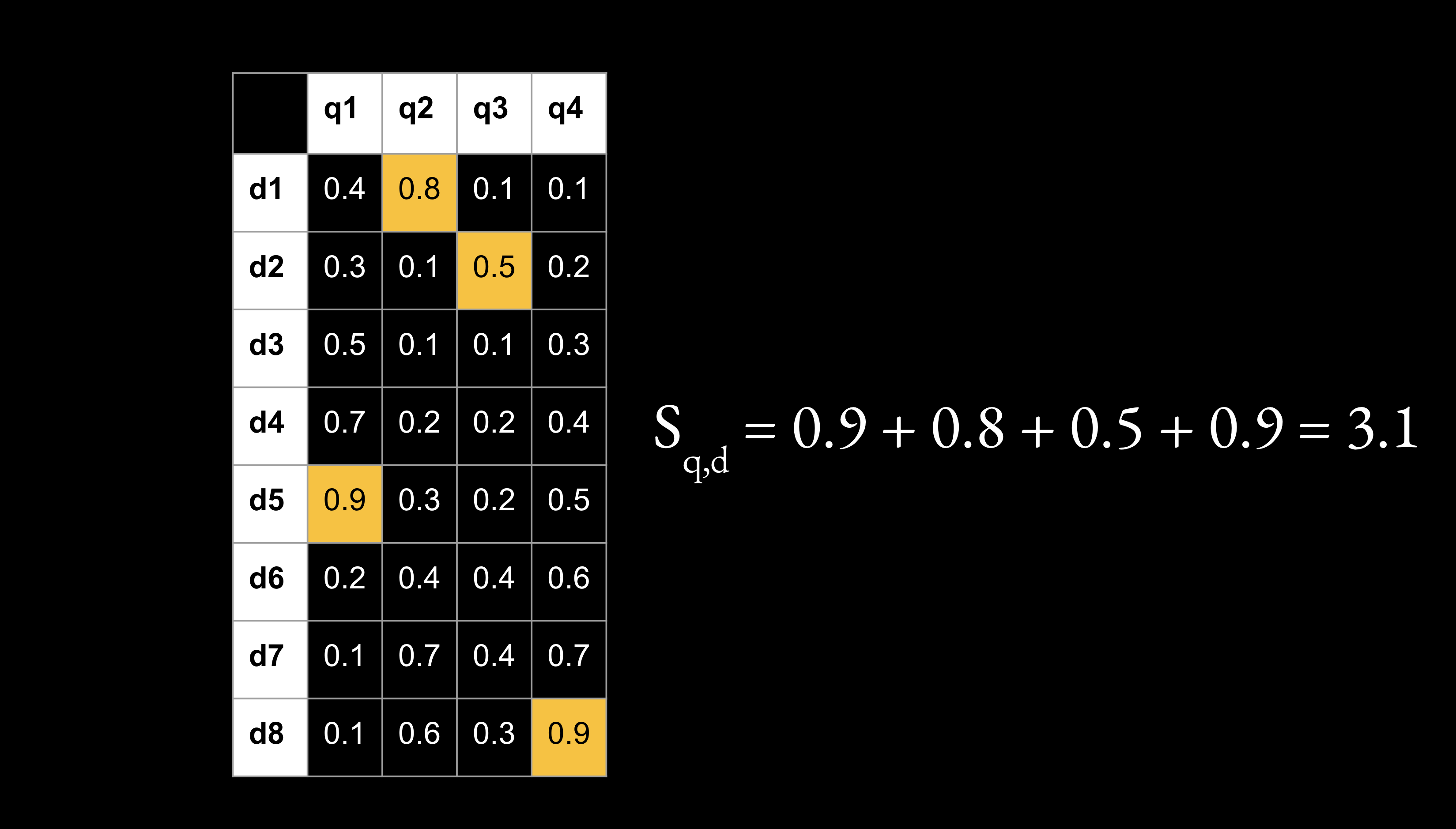
Here is an example of the summation of MaxSim between query and document token embeddings. In this example, we have four query tokens and eight document tokens. For the first query token q1, the highest cosine similarity is with the fifth document token d5. d1 has the maximum cosine similarity for that q2, d2 for q3, and d8 for q4. Adding up these maximum cosine similarities, we get a final relevance score of 3.1. Since there are four tokens, the maximum possible MaxSim value is 4.0.
this interaction mechanism softly searches for each query term tq —in a manner that reflects its context in the query—against the document’s embeddings, quantifying the strength of the “match” via the largest similarity score between tq and a document term td . Given these term scores, it then estimates the document relevance by summing the matching evidence across all query terms.
The query tokens have passed through a transformer model and as such have passed through an attention mechanism so that all tokens attend to all other tokens. So the query itself now has interdependent relationships across tokens. When we’re searching for one token and looking to find the closest document, we’re not just looking to find the closest document to that token in isolation, we’re trying to find the closest document to that token within the context of the entire query. Some contextualized query token embeddings will find strong matches in certain documents, but what we’re looking for is the document for which the total maximum similarity for all query tokens is the largest. You can imagine that as a query gets very long, and the words in the query drift farther apart in meaning, the MaxSim values (before summation) for a document will have high variance.
more sophisticated matching is possible with other choices such as deep convolution and attention layers (i.e., as in typical interaction-focused models),
This reminds me of the Hypencoder paper where they use a neural net for each query that takes as input a document embeddings and outputs a scalar relevance score. This is motivated by the fact that inner product (which is what cosine similarity is) is a linear operation and can thus only linearly separate two groups of vectors (such as embeddings). When your embedding dimension is much smaller than the number of vectors that you have, you can’t separate two groups linearly. In our case, our embedding dimension may be 96 and the number of vectors could be in the millions. Mathematically, you cannot linearly separate such a high number of vectors when they’re in a relatively low-dimensional space.
So you need a complex function because a line doesn’t work, and anytime you need a complex function where it’s more squiggly than a line, a neural net is a good choice!
However, the simplicity of MaxSim has two benefits:
First, it stands out as a particularly cheap interaction mechanism, as we examine its FLOPs in §4.2. Second, and more importantly, it is amenable to highly-efficient pruning for top-k retrieval, as we evaluate in §4.3. This enables using vector-similarity algorithms for skipping documents without materializing the full interaction matrix or even considering each document in isolation. Other cheap choices (e.g., a summation of average similarity scores, instead of maximum) are possible; however, many are less amenable to pruning.
ColBERT’s MaxSim mechanism enables efficient pruning: document tokens are clustered by similarity in vector indexes. At query time, each query token searches only the nearest clusters, skipping irrelevant documents. The “maximum” aggregation makes this possible—you only need the best matches, not exhaustive comparison across all documents.
We’re going to take a look at this paragraph, and then we’re going to look at the code that corresponds to it. Note that this is for a single query, which is what I’m going to focus on.
Given a query q, we compute its bag of contextualized embeddings Eq (Equation 1) and, concurrently, gather the document representations into a 3-dimensional tensor D consisting of k document matrices. We pad the k documents to their maximum length to facilitate batched operations, and move the tensor D to the GPU’s memory. On the GPU, we compute a batch dot-product of Eq and D, possibly over multiple mini-batches. e output materializes a 3-dimensional tensor that is a collection of cross-match matrices between q and each document. To compute the score of each document, we reduce its matrix across document terms via a max-pool (i.e., representing an exhaustive implementation of our MaxSim computation) and reduce across query terms via a summation. Finally, we sort the k documents by their total scores.
So let’s first look at the higher level class which is the IndexScorer. In score_pids, if the query size is 1 (which it is in our case), it’s going to pass the query and the documents to colbert_score_packed.
if Q.size(0) == 1:
    return colbert_score_packed(Q, D_packed, D_mask, config), pids
Inside colbert_score_packed, it removes the unit batch axis of the queries, and makes sure that q and d both have two dimensions. Then it performs the dot product between the two, and we can do this instead of explicitly calling cosine similarity because q and d are both normalized embeddings. The dot product results in a scores tensor that has size number of document tokens x number of query tokens. It then passes these scores into the StridedTensor and it gets back scores_padded and scores_mask which are then passed to colbert_score_reduce.
def colbert_score_packed(Q, D_packed, D_lengths, config=ColBERTConfig()):
    """
        Works with a single query only.
    """

    use_gpu = config.total_visible_gpus > 0

    if use_gpu:
        Q, D_packed, D_lengths = Q.cuda(), D_packed.cuda(), D_lengths.cuda()

    Q = Q.squeeze(0) # removes the unit batch axis

    assert Q.dim() == 2, Q.size()                     # num query tokens x emb dim
    assert D_packed.dim() == 2, D_packed.size()       # num doc tokens   x emb dim

    scores = D_packed @ Q.to(dtype=D_packed.dtype).T  # num doc tokens x num query tokens

    if use_gpu or config.interaction == "flipr":
        scores_padded, scores_mask = StridedTensor(scores, D_lengths, use_gpu=use_gpu).as_padded_tensor()

        return colbert_score_reduce(scores_padded, scores_mask, config)
    else:
        return ColBERT.segmented_maxsim(scores, D_lengths)
scores_padded has shape number of documents x maximum number of tokens in the documents x number of query tokens. So if we have three documents, a maximum of 13 document tokens, and 32 query tokens, scores_padded has shape 3 x 13 x 32.
Finally, colbert_score_reduce is called which takes the maximum of scores_padded across the second dimension (number of document tokens) to leave us with one score for each query token per document.
def colbert_score_reduce(scores_padded, D_mask, config: ColBERTConfig):
    D_padding = ~D_mask.view(scores_padded.size(0), scores_padded.size(1)).bool()
    scores_padded[D_padding] = -9999
    scores = scores_padded.max(1).values

    # flipr code removed for brevity

    return scores.sum(-1)
Taking scores.sum(-1), the summation across the query token dimension, leaves us with one score per document, our desired result.
Relative to existing neural rankers (especially, but not exclusively, BERT-based ones), this computation is very cheap that, in fact, its cost is dominated by the cost of gathering and transferring the pre-computed embeddings. To illustrate, ranking k documents via typical BERT rankers requires feeding BERT k different inputs each of length l = |q| + |di | for query q and documents di , where attention has quadratic cost in the length of the sequence. In contrast, ColBERT feeds BERT only a single, much shorter sequence of length l = |q|. Consequently, ColBERT is not only cheaper, it also scales much better with k as we examine in §4.2.
So, what is involved in that cost of gathering and transferring the pre-computed embeddings? We will look at what they say about offline indexing next.
Instead of applying MaxSim between one of the query embeddings and all of one document’s embeddings, we can use fast vector-similarity data structures to efficiently conduct this search between the query embedding and all document embeddings across the full collection. For this, we employ an off-the-shelf library for large-scale vector-similarity search, namely faiss [15] from Facebook. In particular, at the end of offline indexing (§3.4), we maintain a mapping from each embedding to its document of origin and then index all document embeddings into faiss.
The current implementation in the repo uses a more efficient indexing system, the PLAID index, as opposed to what is written here (indexing “all document embeddings into faiss” and “mantain a mapping from each embeddings to its document of origin”). Instead, the PLAID index uses residual compression with centroids, maintains an Inverted File (IVF) structure that maps centroids to passage IDs, and stores embeddings as compressed residuals relative to centroids.
There’s a lot to unpack in the following section:
Subsequently, when serving queries, we use a two-stage procedure to retrieve the top-k documents from the entire collection. Both stages rely on ColBERT’s scoring: the first is an approximate stage aimed at filtering while the second is a refinement stage. For the first stage, we concurrently issue Nq vector-similarity queries (corresponding to each of the embeddings in Eq ) onto our faiss index. This retrieves the top-k’ (e.g., k’ = k/2) matches for that vector over all document embeddings. We map each of those to its document of origin, producing Nq × k’ document IDs, only K ≤ Nq × k’ of which are unique. These K documents likely contain one or more embeddings that are highly similar to the query embeddings. For the second stage, we refine this set by exhaustively re-ranking only those K documents in the usual manner described in §3.5. In our faiss-based implementation, we use an IVFPQ index (“inverted file with product quantization”). This index partitions the embedding space into P (e.g., P = 1000) cells based on k-means clustering and then assigns each document embedding to its nearest cell based on the selected vector-similarity metric. For serving queries, when searching for the top-k’ matches for a single query embedding, only the nearest p (e.g., p = 10) partitions are searched. To improve memory efficiency, every embedding is divided into s (e.g., s = 16) sub-vectors, each represented using one byte. Moreover, the index conducts the similarity computations in this compressed domain, leading to cheaper computations and thus faster search.
So with that, we have pretty much covered all of the conceptual foundations of ColBERT. To understand the impact of those foundations, we’ll now look at the experimental evaluation section from the paper.
And we’ll explore the four research questions that the ColBERT authors have put forth in this section.
Some training details to prepare the ColBERT retriever: they fine-tune ColBERT models on the MS MARCO and TREC CAR datasets with a learning rate of 3e-6 and a batch size of 32. They fix the number of embeddings per query at 32, meaning that they have 32 tokens per query, and the embedding dimension is 128. The model is trained on a triple of query, positive document and negative document. ColBERT is used to produce a score for each document individually, and is optimized via pairwise softmax cross-entropy loss over the computed scores of the positive and negative document.
Here are two lines from the train function where you can see the loss method, which is cross-entropy loss, and that the labels are just zeros because the document that is positive is first in the batch item (the zero-eth index):
...

labels = torch.zeros(config.bsize, dtype=torch.long, device=DEVICE)

...

loss = nn.CrossEntropyLoss()(scores, labels[:scores.size(0)])
We’ll now dig into the results of their evaluation of the ColBERT architecture vs. existing methods to address the four research questions listed.
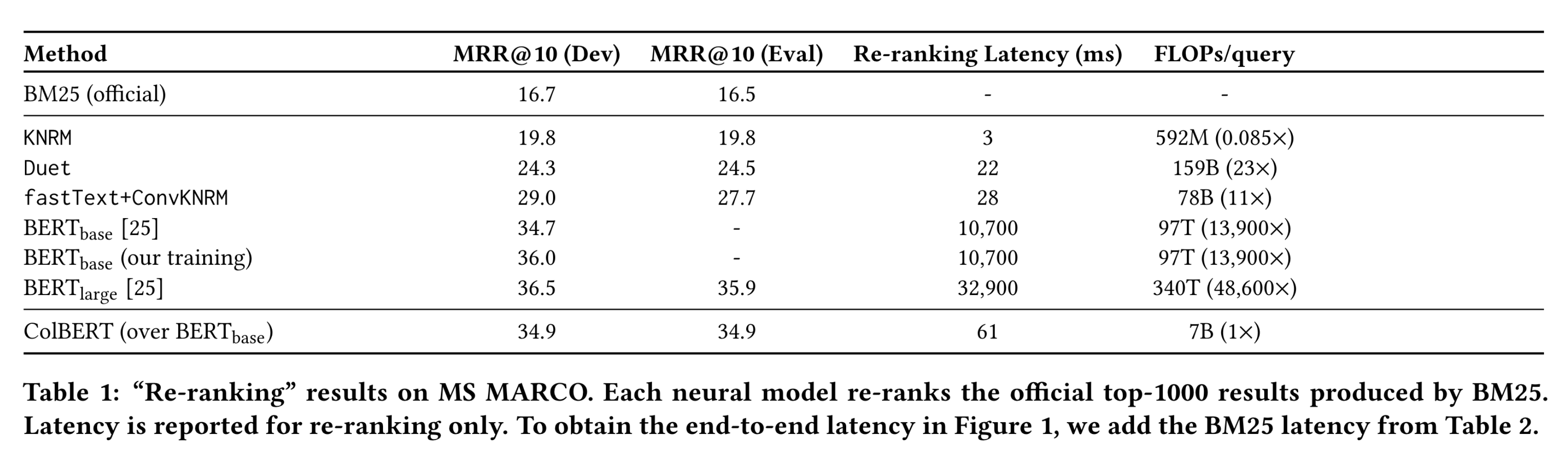
Here are the results for the first type of evaluation where Colbert and other architectures are used to re-rank The top 1000 results produced by BM25, which is full text search. There are three notable takeaways from this table:
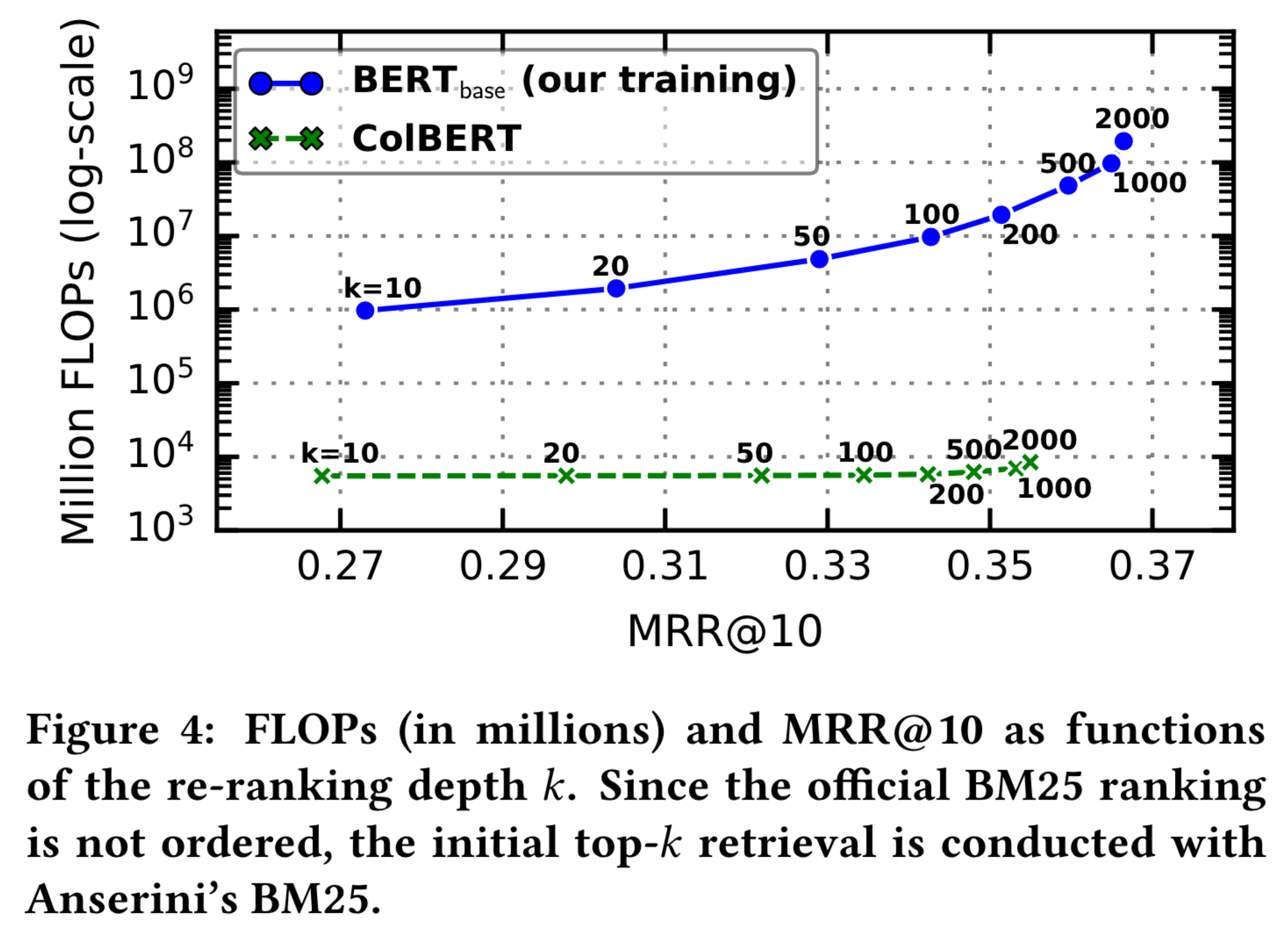
They also compared ColBERT to BERT-base trained on retrieval. In this comparison, they increased the number of documents considered for re-ranking, calculated the FLOPs required to perform the re-ranking and then calculated the retrieval performance. The purple line at the top shows BERT-base, the green line at the bottom shows ColBERT. ColBERT for each value of k (number of documents reranked) requires fewer FLOPs and is comparable in retrieval performance. Most importantly, ColBERT scales much better than BERT-base as the number of document candidates considered increases from 10 to 2000. ColBERT stays within the same order of magnitude for FLOPs whereas BERT-base FLOPs increase by two orders of magnitude.
Next, we’ll look at their full retrieval results where they retrieve the top 1000 documents from the 8.8 million document MS Marco Corpus.
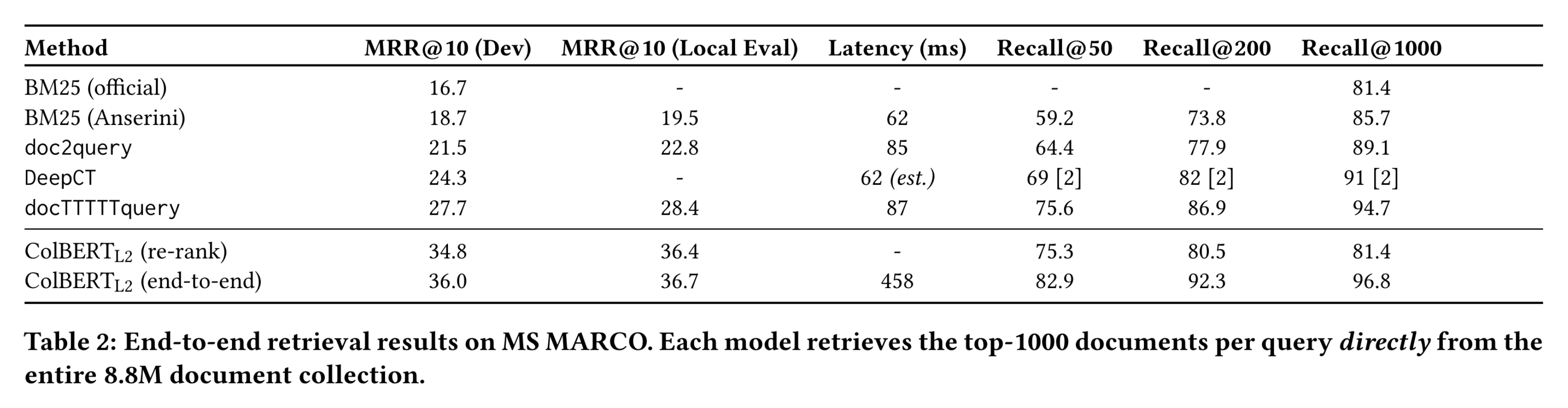
What immediately jumps off the page here is the MRR improvement that ColBERT provides, twice that of the Anserini BM25 method, which is an excellent baseline. However, ColBERT has about 5-8 times the latency of these other methods–that could be justifiable given the increased improvement. ColBERT (end-to-end) has the best Recall across all methods.
Next, we’ll look at some of the ablation studies that they performed, which to me are the most exciting results.
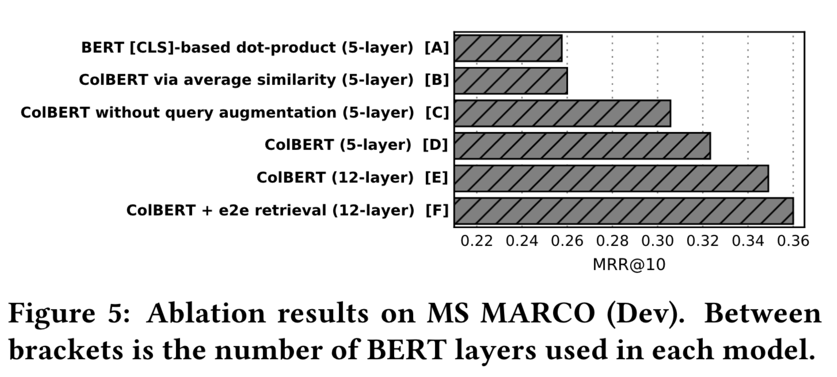
This figure is really interesting, and there’s a lot to unpack here. I think it serves as a really comprehensive summary of the main architectural decisions that they’ve made in this work.
Models A through E are used in a re-ranking setting. The first comparison we’ll look at is between model A and model D. Model A is a BERT model, and it takes the CLS token embedding representation for query and document and performs an inner product between them to calculate similarity for re-ranking, which achieves an MRR@10 of about 0.26 which is 6 points fewer than a 5-layer ColBERT model. So, fine grained, token-wise embedding interaction with ColBERT is yielding better results than a single vector interaction with BERT. This is a confirmation of the fundamental concept behind late interaction.
The second comparison is between model B and model D. Model B is using average similarity, and model D is using the MaxSim operator. Model D again has about a 6 point increase in MRR. This validates the second fundamental concept behind late interaction: the MaxSim operator.
The third comparison is between Model C and Model D. In Model C, the query is not padded to 32 tokens with [MASK] tokens. Model D uses query augmentation (it pads to 32 with [MASK] tokens) and has a 2 point increase in MRR showing that these [MASK] tokens, which carry semantic meaning in embedding space, improve the model’s ability to find relevant documents given a query.
The final comparison is between Model E and Model F. Model E is ColBERT used as a re-ranker for the top 1000 documents retrieved by full-text search. Model F is ColBERT used for end-to-end retrieval using a vector similarity index to cluster documents before retrieval. Using ColBERT end-to-end gives another boost to performance.
Something to keep in mind is that BERT requires you to pass in the query and document embedding one pair at a time. For one query, you have to do a thousand forward passes if you have a thousand documents that you want to compare it to. Whereas ColBERT, because of late interaction, can utilize vector similarity indexes because documents are indexed offline, and the interaction calculation is much quicker because you are considering fewer candidate documents—the documents that are close to the query token embeddings via the clusters created by the indexing process.
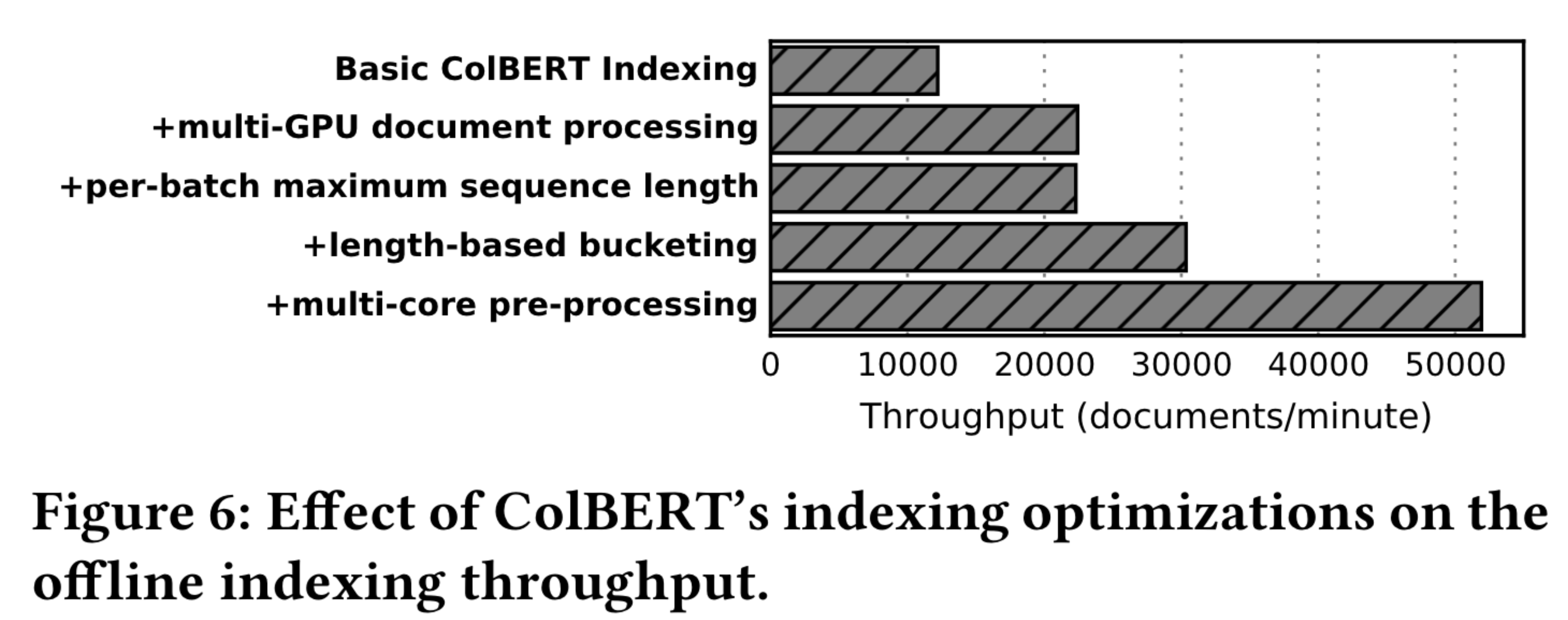
I’ll start by showing figure 6, where it shows that on top of basic ColBERT indexing, adding these optimizations increases the throughput, which means it increases the number of documents that are processed each minute. The two that I’ll highlight here is that length-based bucketing, which we saw in detail, and per-batch maximum sequence length, where they pad all items in the batch to the maximum document length, both improve the throughput.
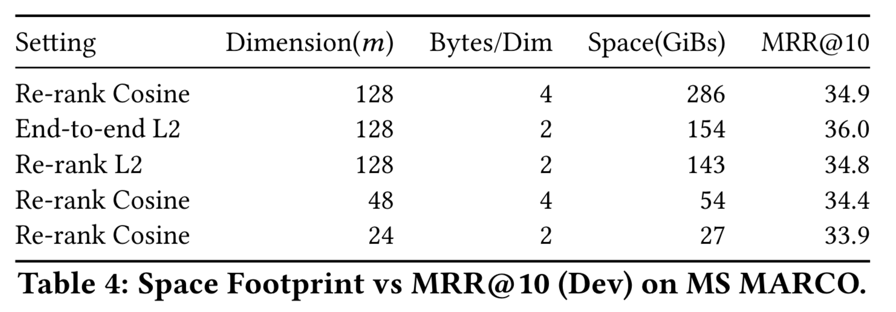
This table shows the space footprint and MRR@10 for different settings, dimensions, and bytes per dimension. The most space-effcient setting, re-ranking with cosine similarity with 24-dimensional vectors stored as 2-byte floats, which takes up 27 GB, is only 1% worse in MRR@10 than the most space-consuming one which takes up 286 GB.
The body of the ColBERTv1 paper is only about 9 pages long, but it is incredibly information dense. What I thought would be a 1-day foray turned into a 6-day deep dive. I found it helpful to interleave twitter conversations with core concepts from the paper, as casual conversations are often more accessible, and equally impressive as formal work.
As a new canonical ColBERT maintainer I wanted to ground myself in the first principles of late interaction. There are three key elements involved:
Encoding queries and documents separately allows for offline document indexing, and delays the interaction to the end of the architecture. Offline indexing and MaxSim both unlock pruning in their own ways. Vector-similarity indexes, through clustering, eliminate low-relevance documents from consideration before the interaction takes place. MaxSim eliminates low-relevance tokens during the interaction.
MaxSim is further enhanced by query augmentation, as meaningful [MASK] tokens are introduced in the query to improve the chance of matching relevant terms in the document.
That the most space-efficient setting is only 1% less performant than the most space-consuming setting foreshadows the compression opportunities realized in the PLAID paper.
With these foundations reinforced, I’ll revisit the ColBERTv2 and PLAID papers next, and will continue to concretely witness the concepts at play in the repo’s codebase.